Applications of Differentiation: Curve Sketching
Calculus techniques can be applied to a wide variety of problems in real life. We consider many examples in this chapter. In each case, we construct a function as a mathematical model of some problem and then analyse the function and its derivatives to gain information about the original problem. Our principal method for analysing a function will be to sketch its graph. For this reason, we devote the first part of the chapter to curve sketching.
Describing Graphs of Functions
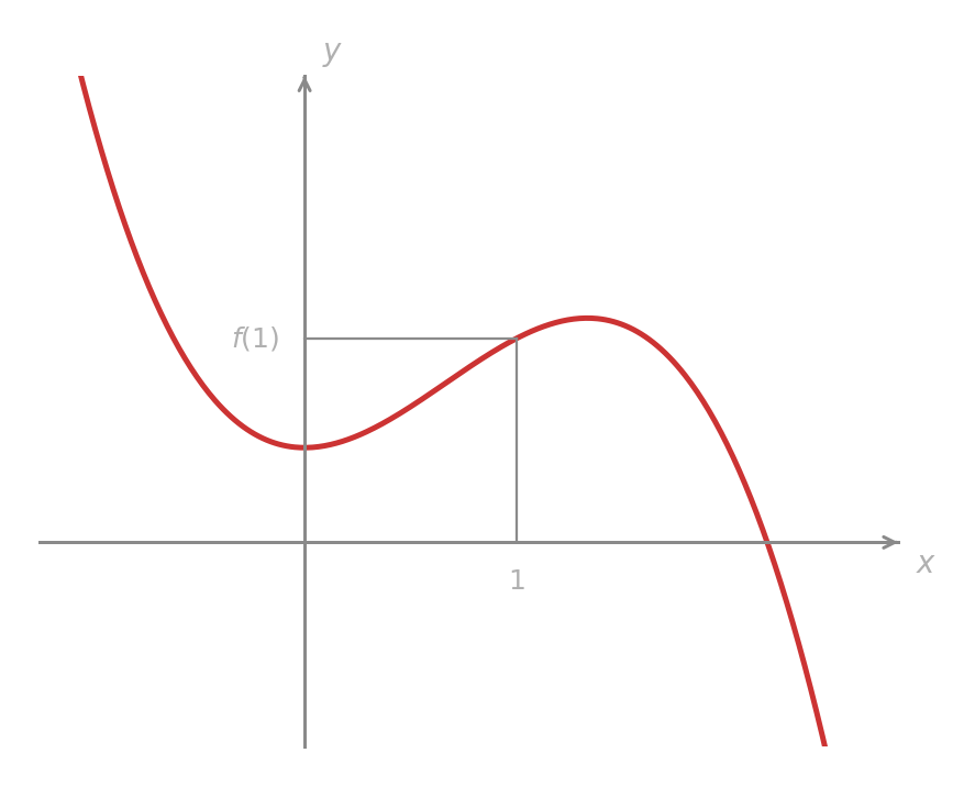
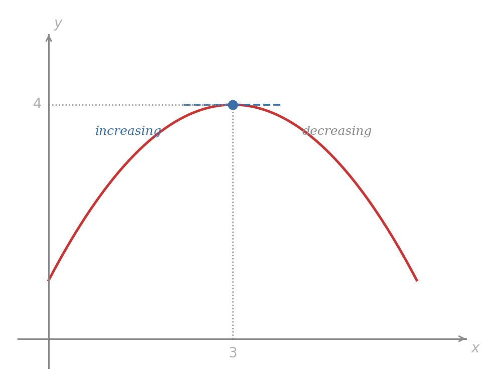
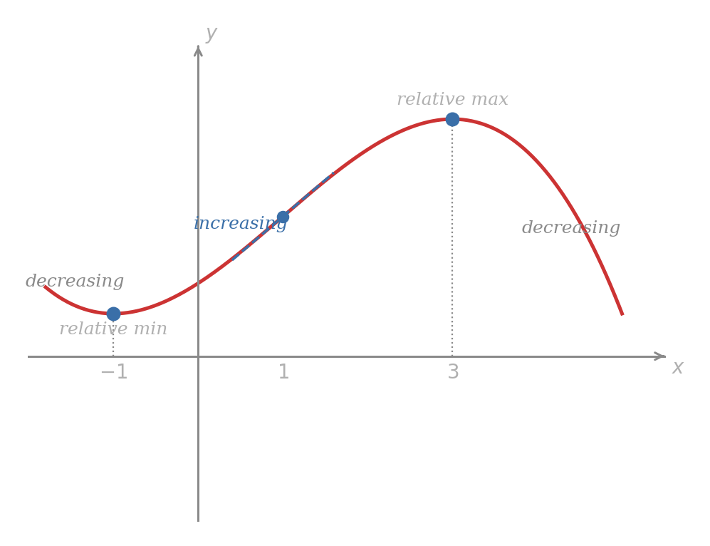
Let’s examine the graph of a typical function, such as the one shown in the figure below, and introduce some terminology to describe its behaviour. First, observe that the graph is either rising or falling, depending on whether we look at it from left to right or from right to left. To avoid confusion, we shall always follow the accepted practice of reading a graph from left to right.
Let’s now examine the behaviour of a function in an interval throughout which it is defined.
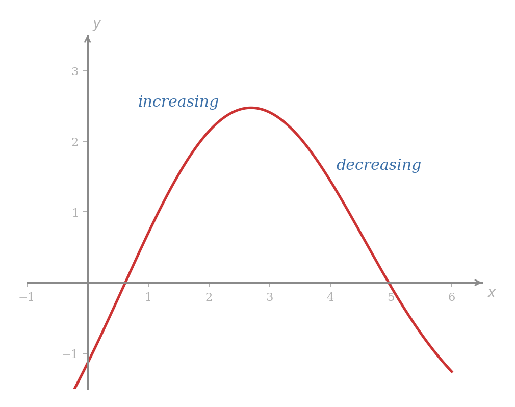
We say that a function is increasing in an interval if the graph continuously rises as goes from left to right through the interval. That is, whenever and are in the interval with , we have . We say that is increasing at provided that is increasing in some open interval on the -axis that contains the point .
We say that a function is decreasing in an interval provided that the graph continuously falls as goes from left to right through the interval. That is, whenever and are in the interval with , we have . We say that is decreasing at provided that is decreasing in some open interval that contains the point .
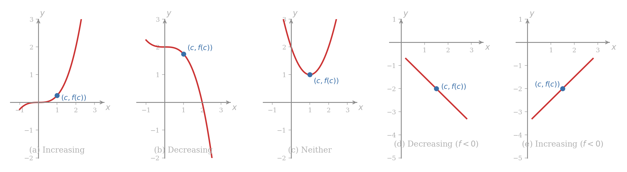
The figure below shows graphs that are increasing and decreasing at . Observe in panel (d) that when is negative and is decreasing, the values of become more negative. When is negative and is increasing, as in panel (e), the values of become less negative.
The visual reading of increasing and decreasing aligns with the slope of the tangent line from Lesson 2PM. A positive derivative makes the graph rise as we read from left to right, while a negative derivative makes the graph fall. A horizontal tangent can occur at a single point without changing the overall rise or fall nearby.
Problem 49
Suppose a function is increasing on and decreasing on . Describe what happens to the graph as moves from left to right through these two intervals. What sign would you expect the tangent slopes to have on each interval?
Problem 50
A graph passes through the points , , , and in that order, with the curve falling from to and rising from to . On which interval is the function decreasing? On which interval is it increasing? What happens at ?
Extreme Points
A relative extreme point or an extremum of a function is a high point or low point compared with nearby points on the graph. We distinguish the two possibilities in an obvious way.
A relative maximum point is a point on the graph whose height is at least as large as the heights of nearby points. A relative minimum point is a point on the graph whose height is at most as large as the heights of nearby points.
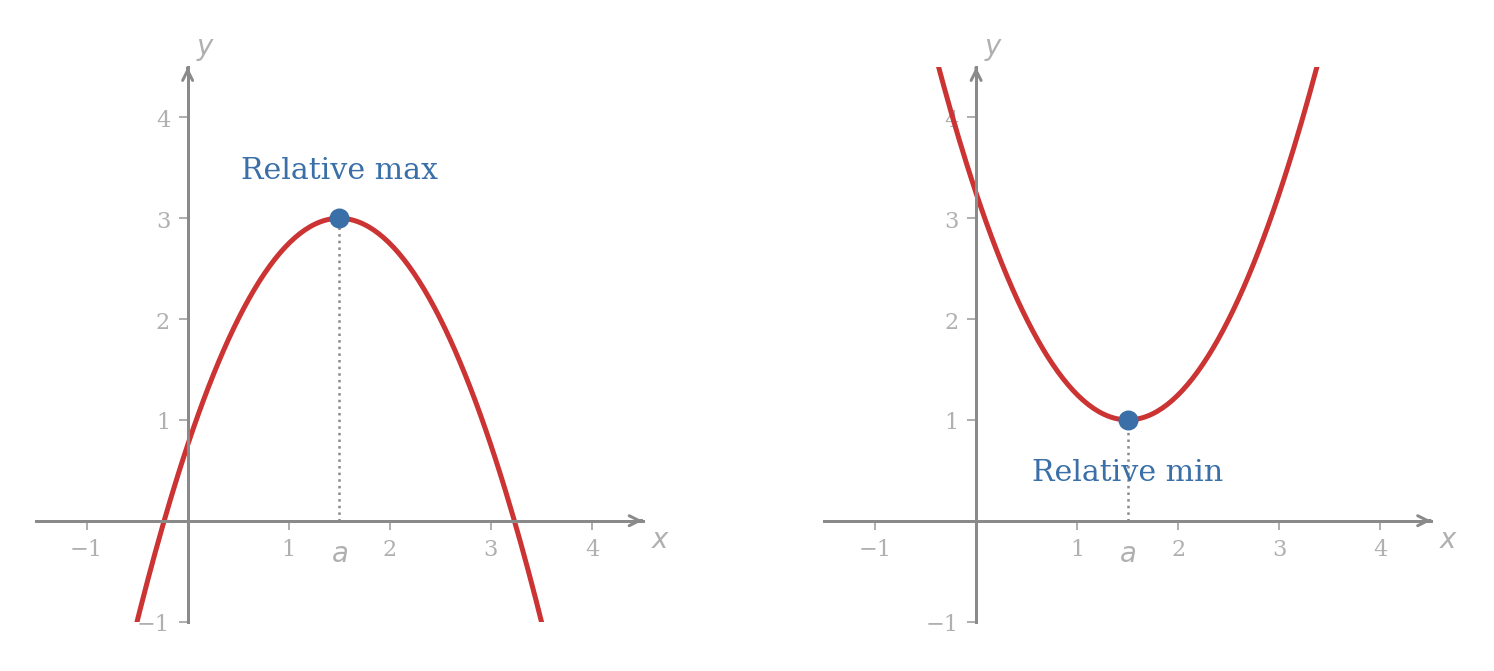
The adjective relative in these definitions indicates that a point is maximal or minimal relative only to nearby points on the graph. The adjective local is also used in place of relative. A change from increasing to decreasing gives a relative maximum, and a change from decreasing to increasing gives a relative minimum.
The maximum value (or absolute maximum value) of a function is the largest value that the function assumes on its domain. The minimum value (or absolute minimum value) of a function is the smallest value that the function assumes on its domain.
Functions may or may not have maximum or minimum values. However, a continuous function whose domain is a closed interval of the form always has both a maximum and a minimum value.
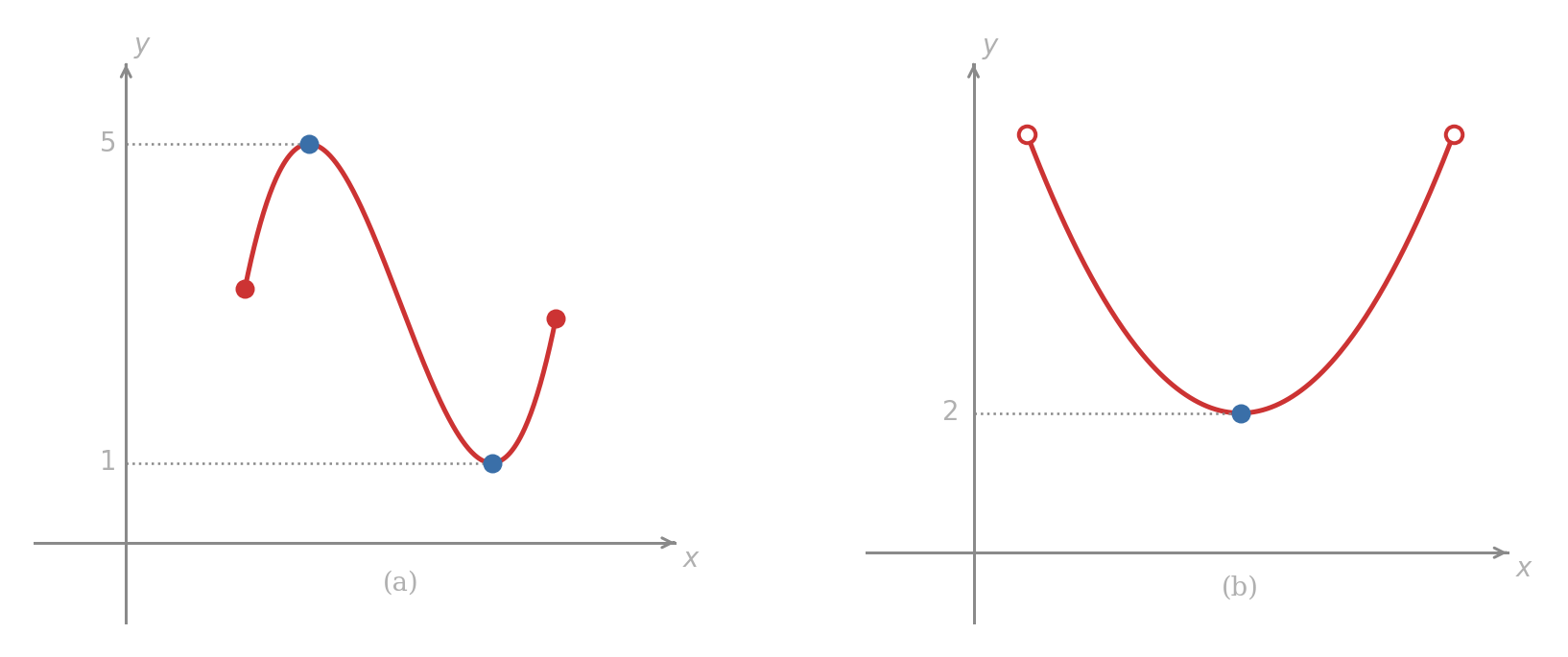
Maximum values and minimum values of functions usually occur at relative maximum points and relative minimum points, as seen in panel (a) above. However, they can occur at endpoints of the domain. If so, we say that the function has an endpoint extreme value (or endpoint extremum).
Relative maximum points and endpoint maximum points are higher than any nearby points. The maximum value of a function is the -coordinate of the highest point on its graph. The highest point is called the absolute maximum point. Similar considerations apply to minima.
Problem 51
A graph has a high point at , a low point at , and another high point at . The highest of all values shown occurs at , while the lowest of all values shown occurs at the left endpoint of the graph. Identify the -coordinates of the relative maximum points, the relative minimum point, the absolute maximum point, and the absolute minimum point.
Problem 52
On the closed interval , a continuous function has values , , , and , and no other higher or lower points occur. Give the maximum value, the minimum value, the absolute maximum point, and the absolute minimum point.
Real-World Applications of Extrema
The mathematical definitions of increasing, decreasing, and extrema directly model behaviour in applied contexts. Finding these points allows us to determine the optimal conditions of a physical, biological, or economic system.
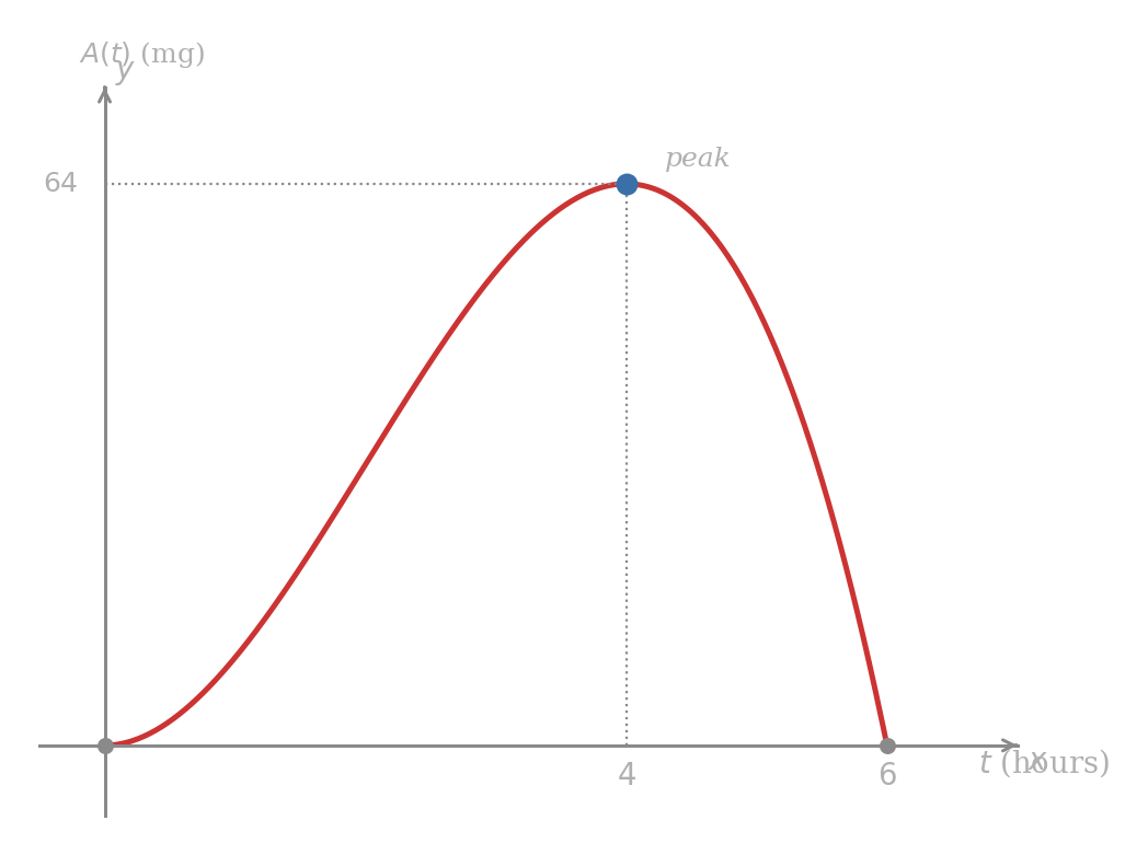
When a drug is injected intramuscularly (into a muscle), the concentration of the drug in the veins has the time-concentration curve shown below. We can describe this graph using the terms introduced previously.
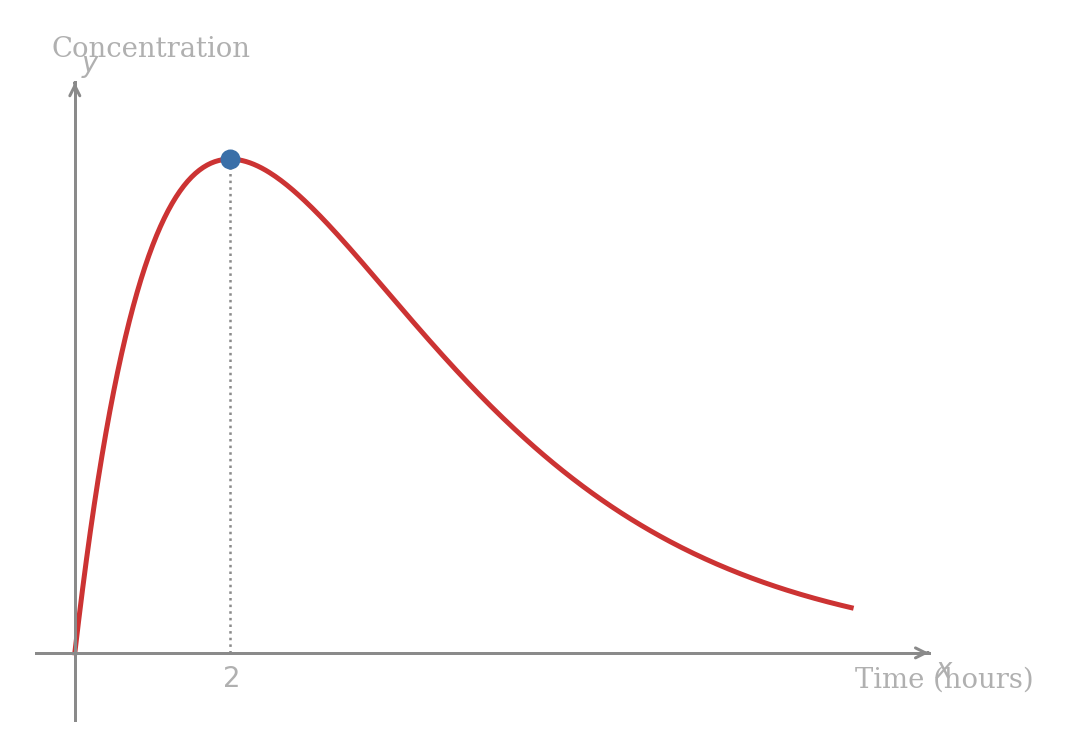
Initially (when ), there is no drug in the veins. When the drug is injected into the muscle, it begins to diffuse into the bloodstream. The drug concentration in the veins increases until it reaches its absolute maximum value at hours.
After this time, the concentration begins to decrease as the body’s metabolic processes remove the drug from the blood. Eventually, the drug concentration decreases to a level so small that, for all practical purposes, it is zero. The peak at represents the relative and absolute maximum of this model.
Problem 53
Consider the drug concentration model from the previous example. During which interval of time is the concentration of the drug strictly increasing? During which interval is it strictly decreasing?
A British manufacturer models the profit from producing and selling thousand electric kettles. The profit function, shown below, accounts for both the revenue generated from sales and the costs associated with production.
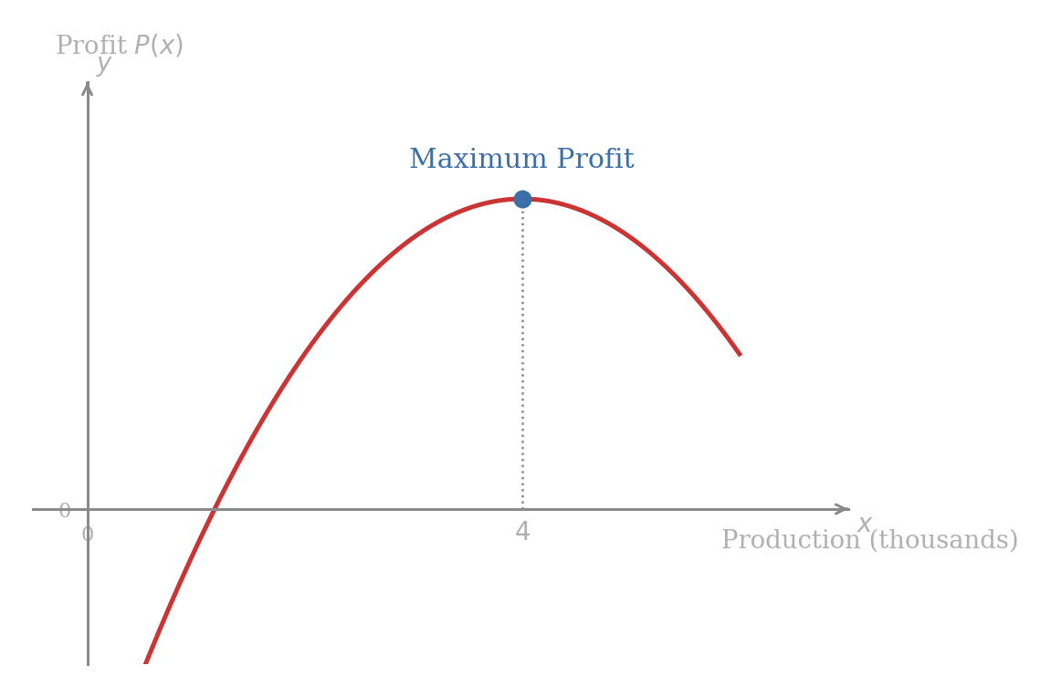
At low production levels, the profit is negative (a loss) because the initial fixed overhead costs outweigh the revenue. As production increases, increases, eventually turning positive and crossing the break-even point.
The profit continues to rise until production reaches thousand units. At this point, the profit achieves an absolute maximum. If production is pushed beyond this level, inefficiencies and escalating marginal costs cause the profit to decrease. The relative maximum at represents the best production target for the manufacturer.
Problem 54
In the profit model above, what does it mean, in business language, for to be increasing before ? What does it mean for to be decreasing after ? Why is the production level the manufacturer would prefer if the model is trusted?
Problem 55
A ball is thrown vertically upward from the ground. Its height in metres after seconds is modelled by a curve that opens downward.
- Describe the physical meaning of the function increasing.
- What physical event corresponds to the relative maximum of ?
- Describe the physical meaning of the function decreasing.
Changing Slope
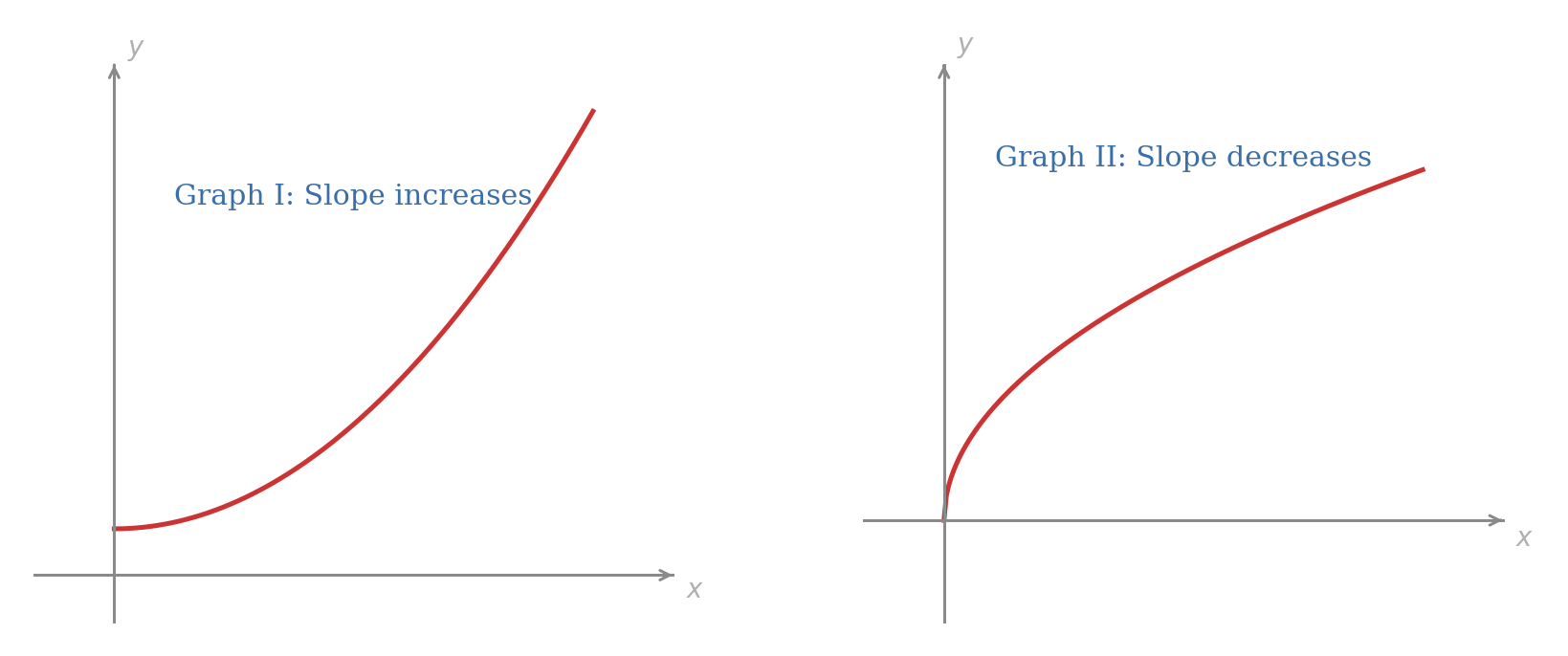
Another feature of a graph is the way its slope changes as we look from left to right. The two graphs shown below are both increasing, but they increase in different ways.
Graph I, which could describe a quantity like compound interest or population growth, is steeper on the right than on the left. That is, the slope of graph I increases as we move from left to right. A newspaper description of graph I might read, “The quantity rose at an increasing rate.”
In contrast, the slope of graph II decreases as we move from left to right. Although the quantity is rising, the rate of increase declines throughout. That is, the slope becomes less positive. The media might say, “The quantity rose at a decreasing rate.”
Problem 56
A railcard app’s subscribers increase from to in the first month, from to in the second month, and from to in the third month. Is the subscriber count increasing? Is it increasing at an increasing rate or at a decreasing rate over these months?
Problem 57
A tank is being filled. During three equal time intervals, the amount of water increases by litres, then litres, then litres. Is the amount of water increasing or decreasing? Is the slope increasing or decreasing?
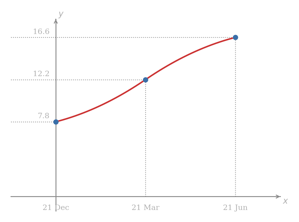
The daily number of hours of daylight in London increases from about hours on 21 December to about hours on 21 March, and then to about hours on 21 June. From 21 December to 21 March, the daily increase is greater than the previous daily increase, and from 21 March to 21 June, the daily increase is less than the previous daily increase.
If we draw a possible graph of the number of hours of daylight as a function of time, the first part of the graph is increasing at an increasing rate. The second part of the graph is increasing at a decreasing rate.
Problem 58
In the daylight example, the function is increasing throughout the whole interval from 21 December to 21 June. Why does that not mean the slope is increasing throughout the whole interval?
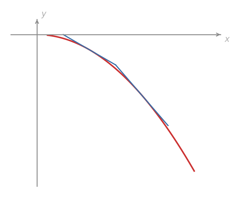
Recall that when a negative quantity decreases, it becomes more negative. (Think about the temperature outside when it is below zero and the temperature is falling.) So if the slope of a graph is negative and the slope is decreasing, the slope is becoming more negative, as seen below. This technical use of the term decreasing runs counter to our intuition, because in popular discourse, “decrease” often means to become smaller in magnitude.
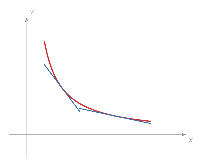
Similarly, the curve below is becoming “less steep” in a nontechnical sense (since steepness refers to the magnitude of the slope). However, the slope of the curve is increasing because it is becoming less negative. The popular press would probably describe the curve as decreasing at a decreasing rate, because the rate of fall tends to taper off. Since this terminology is potentially confusing mathematically, we prefer simply saying the slope is increasing.
Problem 59
Compare two falling graphs. In the first, tangent slopes at equally spaced points are approximately , , and . In the second, the slopes are approximately , , and . For each graph, decide whether the slope is increasing or decreasing.
Problem 60
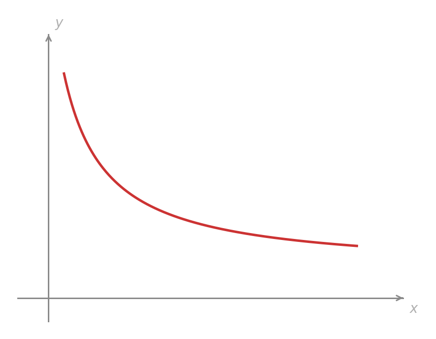
Does the slope of the curve shown below increase or decrease as increases?
Concavity
The “increasing at an increasing rate” and “increasing at a decreasing rate” ideas may also be described in geometric terms using tangent lines.
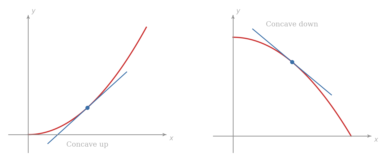
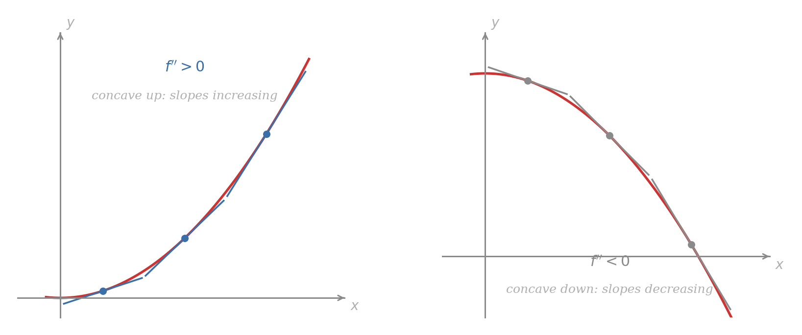
We say that a function is concave up at if there is an open interval on the -axis containing throughout which the graph of lies above its tangent line. Equivalently, is concave up at if the slope of the graph increases as we move from left to right through .
We say that a function is concave down at if there is an open interval on the -axis containing throughout which the graph of lies below its tangent line. Equivalently, is concave down at if the slope of the graph decreases as we move from left to right through .
Problem 61
Suppose the tangent slopes stay positive and increase as moves left to right through an interval. Is the graph increasing or decreasing there? Is it concave up or concave down?
Problem 62
Suppose the tangent slopes decrease as moves left to right through an interval, passing from positive values to negative values. Is the slope increasing or decreasing? Is the graph concave up or concave down?
Inflection Points
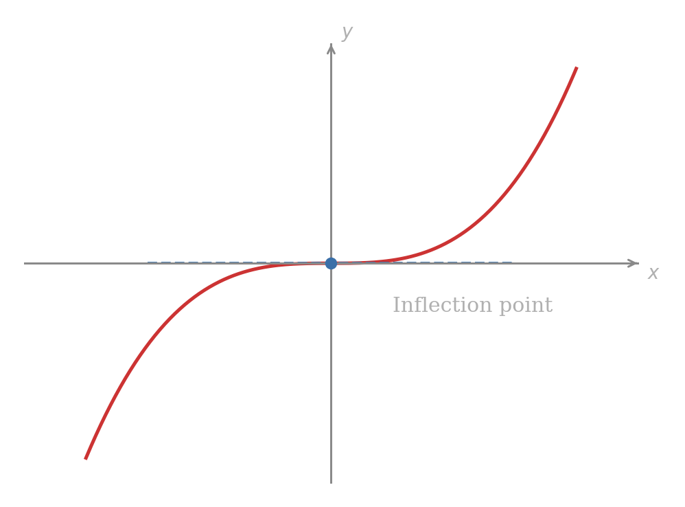
An inflection point is a point on the graph of a function at which the function is continuous and at which the graph changes from concave up to concave down or vice versa.
In the smooth examples considered here, the graph crosses its tangent line at an inflection point. The continuity condition means that the graph cannot break there.
Problem 63
A continuous graph is concave down for and concave up for . What kind of point occurs at ? What additional information would you need in order to name the point itself as an ordered pair?
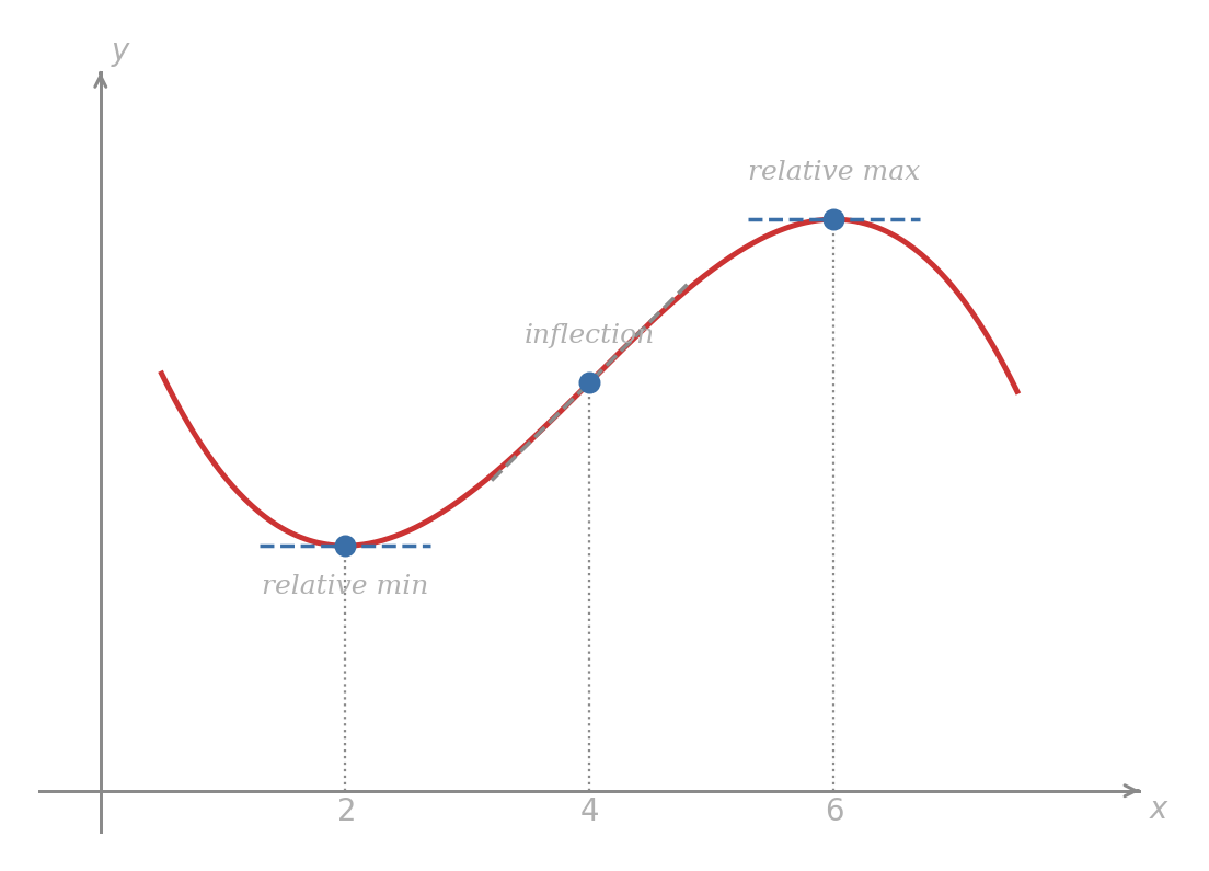
Use the terms defined earlier to describe the graph shown below.
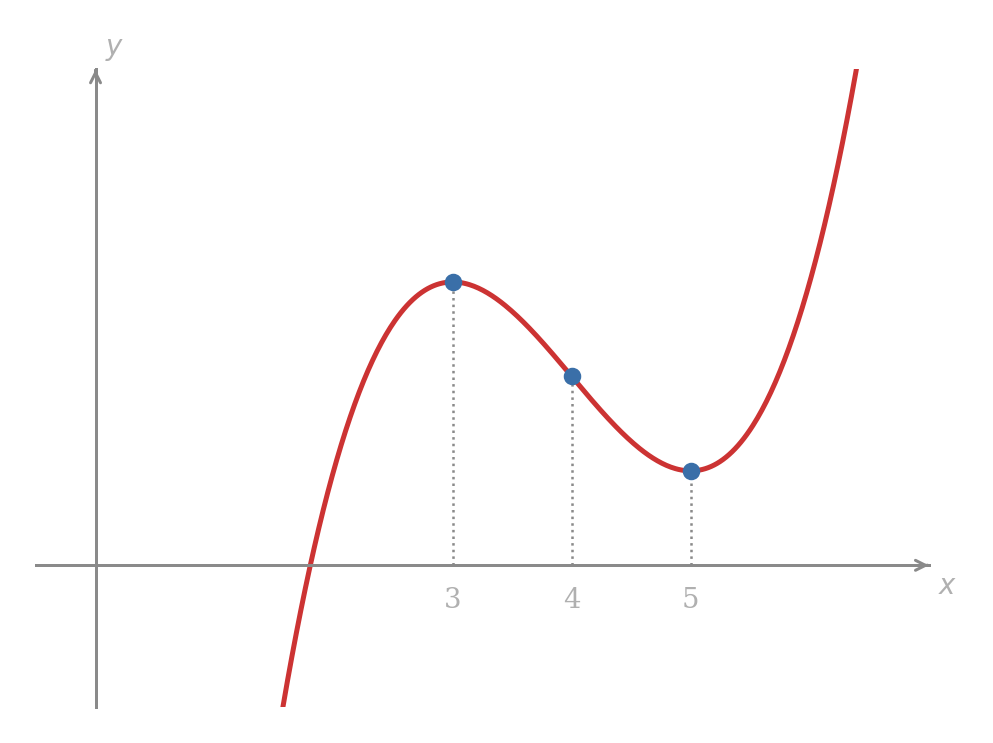
- For , is increasing and concave down.
- Relative maximum point at .
- For , is decreasing and concave down.
- Inflection point at .
- For , is decreasing and concave up.
- Relative minimum point at .
- For , is increasing and concave up.
Problem 64
For a graph with the same shape as the example above, explain why is not a relative maximum or relative minimum even though it is an important point of the graph.
Problem 65
Suppose a graph is decreasing and concave down on , then decreasing and concave up on . What happens at ? Does the graph have to stop decreasing there?
The First- and Second Derivative rules
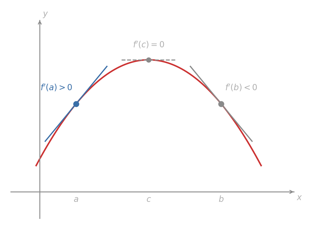
The preceding sections built a vocabulary for graphs: increasing, decreasing, concave up, concave down, relative extrema, inflection points. Since Lesson 2PM identified as the tangent slope, the sign of lets us locate increasing and decreasing intervals without constructing the graph first.
If throughout an interval, then is increasing on that interval.
If throughout an interval, then is decreasing on that interval.
When , neither interval rule applies at that input alone: the tangent is horizontal, and the function might have a relative maximum, a relative minimum, or neither at . The zero marks a candidate worth examining in context.
Sketch the graph of a function satisfying all of the following:
-
-
for , , for
We begin with the single concrete point and draw a horizontal tangent there since . By the first derivative rule, is increasing for every and decreasing for every . The graph rises to and falls away from it on both sides, making a relative maximum.
Problem 66
A function satisfies , for , , and for . Use the first derivative rule to determine whether is a relative maximum, a relative minimum, or neither, and sketch a rough graph consistent with these conditions.
Problem 67
A function satisfies on , , on , , and on . Identify all -coordinates at which relative extrema occur and all intervals on which is increasing or decreasing. Does the zero of at produce an extremum?
The second derivative measures how the tangent slope changes. Thus the sign of gives the concavity.
If throughout an interval, then is concave up on that interval.
If throughout an interval, then is concave down on that interval.
When , the rule gives no information; the function may be concave up, concave down, or have an inflection point there.
When the signs of and hold throughout an interval, they pin down both the monotonicity and the concavity there. The four combinations cover all qualitatively distinct behaviours.
| on the interval | on the interval | behaviour of |
|---|---|---|
| positive | positive | increasing, concave up |
| positive | negative | increasing, concave down |
| negative | positive | decreasing, concave up |
| negative | negative | decreasing, concave down |
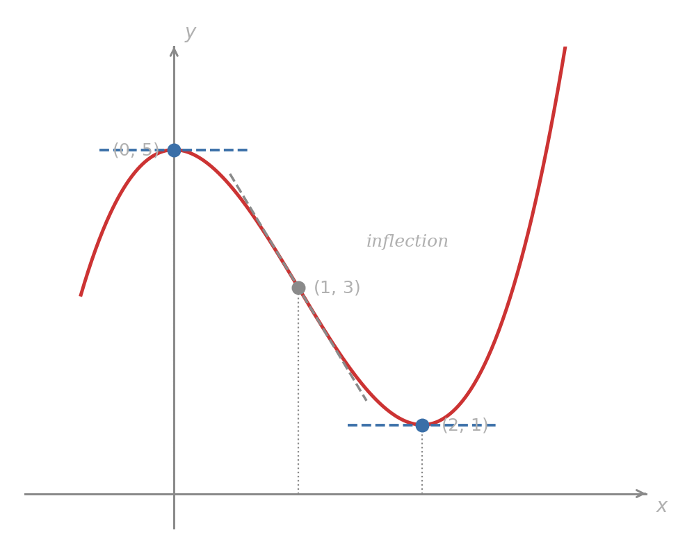
Sketch the graph of a function with the following properties:
-
The points , , and lie on the graph.
-
and .
-
for , , for .
The second derivative rule, combined with the zero-derivative conditions, determines the character of each key point. At : and (since ), so a horizontal tangent on a concave-up curve — this is a relative minimum. At : and (since ), so a horizontal tangent on a concave-down curve — a relative maximum. At : concavity changes from up to down, so is an inflection point.
Between the two extrema the function increases through a concave-up bowl (for ) into a concave-down arch (for ), crossing through the inflection point at where the transition occurs.
Problem 68
Use the first and second derivative rules to analyse on .
- Compute and .
- Find the intervals on which is increasing and decreasing.
- Find the intervals on which is concave up and concave down, and locate the inflection point.
- What does the inflection point say about how the rate of change of is itself changing?
Problem 69
A manufacturer’s profit is modelled by , where is thousands of units produced.
- Use the first derivative rule to find the intervals on which is increasing and decreasing.
- Identify the production level that gives the relative maximum profit.
- Compute and use the second derivative rule to confirm the point is a maximum rather than a minimum.
The applied examples in the Real-World Applications section raised a question without the tools to answer it: how do we know where the drug concentration peaks or where profit is maximised? Away from endpoints, the first derivative rule provides the mechanism: a transition from increasing to decreasing or from decreasing to increasing is detected by the sign of around a critical input. When and , concavity then confirms a local maximum; when , it confirms a local minimum. This turns the descriptive vocabulary above into computations, setting up the systematic optimisation treated in subsequent lessons.
Connections between the Graphs of and
Think of as the slope function for : the -coordinate on the graph of at any input is the slope of at that input. Every qualitative feature of ‘s shape — whether it is rising or falling, whether that rise accelerates or slows — leaves a direct trace on the graph of .
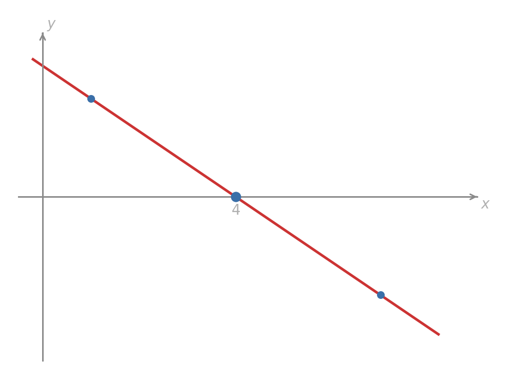
The function is graphed below together with the slope at several points.
The slopes are decreasing as we move from left to right: steeply positive at , zero at , and steeply negative at . So is a decreasing function. Computing , whose graph is shown below.
The -values of match the slopes on the parabola exactly: positive for , zero at , negative for . The parabola is the shape of a typical revenue curve; the graph of is the corresponding marginal revenue curve, whose zero at identifies the revenue-maximising output.
Marginal cost was introduced in Lesson 2AM as the slope of a linear cost function — a fixed constant for every unit. Here plays the same role for a nonlinear revenue model, but now varying continuously with . Setting the marginal revenue to zero and solving recovers the output that maximises revenue, a calculation pattern that recurs throughout the optimisation lessons ahead.
Problem 70
For , compute , , and algebraically. Confirm that each value matches the sign and direction of the corresponding tangent line in the figure. At which inputs is increasing? At which is it decreasing? What determines the production level a revenue-maximising firm would choose?
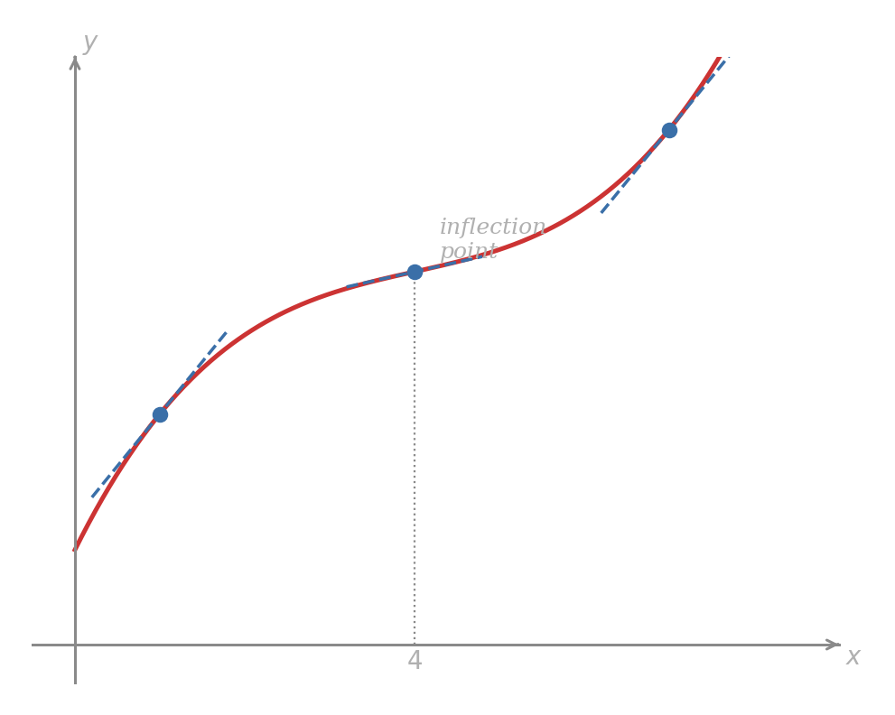
The function models a total cost curve whose slope — the marginal cost — first decreases and then increases. Several slopes are marked on the graph of below.
The derivative is , an upward-opening parabola graphed below.
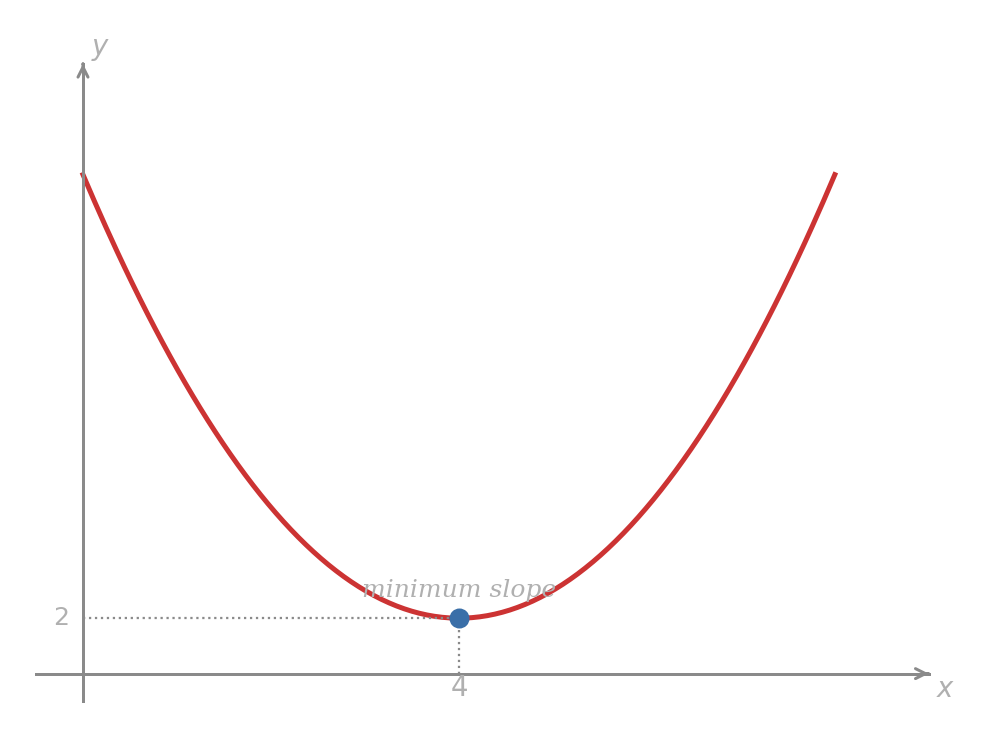
The -values on the graph of decrease and then increase, reaching their minimum at . Since , we have , and changes sign there from negative to positive. By the second derivative rule, is the inflection point of — where the cost curve transitions from concave down to concave up. The inflection point of the cost curve coincides exactly with the input at which the marginal cost curve is minimised.
Problem 71
For :
- Compute and .
- Find the input at which is minimised by solving .
- Confirm that this input is the inflection point of by checking the sign of on either side.
- What is the minimum value of the marginal cost? Is it zero? What would it mean economically if it were zero?
The graph of is shown below.
- What is the slope of at ?
Since , the graph of has slope at .
- Describe how changes on .
The values of are positive and decreasing as increases from to .
- Describe the shape of on .
Since throughout this interval, is increasing there. Since is decreasing on this interval, the slope of is decreasing, which by the Concavity definition means is concave down on .
- For what values of does have a horizontal tangent?
Horizontal tangents occur where . From the graph, these are and .
- Explain why has a relative maximum at .
Just to the left of , , so is increasing; just to the right, , so is decreasing. By the Relative Maximum definition, transitions from increasing to decreasing at and therefore has a relative maximum there.
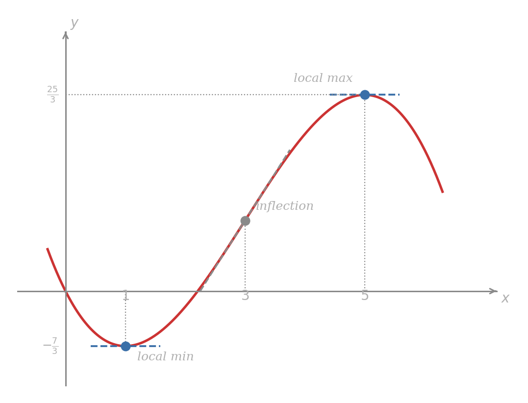
A graph of consistent with these conditions is shown below.
Problem 72
Referring to the graph of in the example above:
- On which interval is increasing? On which is it decreasing?
- Use the sign of on each side of to decide whether has a relative maximum or a relative minimum there.
- On which interval is concave up? On which is it concave down? Identify the inflection point.
Problem 73
A function satisfies on , , on , and for all . Without computing explicitly, describe its shape completely: identify its monotonicity, concavity, and all -coordinates at which extrema occur.
The First Derivative Test
Knowing that pins down a candidate for an extremum, but not every such candidate is one. The sign of on either side of decides the issue: if is positive to the left and negative to the right, the graph arches over , giving a local maximum; if the signs reverse, the graph dips through , giving a local minimum; if keeps the same sign on both sides, the function does not reverse direction and there is no extremum at . The input in each case is a critical number.
A number in the domain of is a critical number of if or if does not exist. The point on the graph is called a critical point.
The first derivative rule ensures that every local extreme point occurs at a critical number. The converse fails: a critical number is a candidate, and whether it is an extremum depends on the sign change of there.
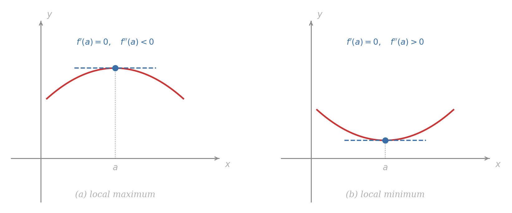
The four panels below display each possibility in the common case .
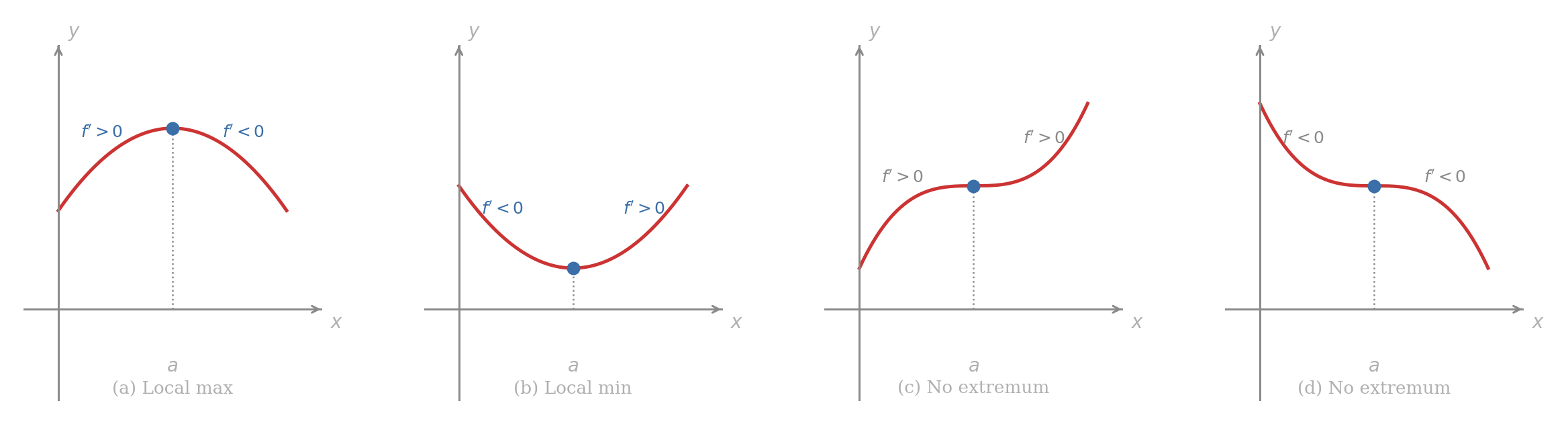
Suppose is a critical number of , and suppose has a definite sign on each side of near .
-
If changes from positive to negative at , then has a local maximum at .
-
If changes from negative to positive at , then has a local minimum at .
-
If does not change sign at , then has no local extremum at .
To implement the test, first locate the critical numbers: solve , and also record any inputs where does not exist while itself is defined. These critical numbers divide the real line into open intervals. On each interval the sign of is constant for the examples in this lesson. A sign chart records these signs by factoring and checking the sign of each factor at a sample from each interval; the sign of the product gives the sign of and hence the direction of on that interval.
For , the derivative is for and for , but does not exist because the left and right slopes disagree. The input is still a critical number because is defined.
The sign of changes from negative on the left of to positive on the right of , so the first derivative test gives a local minimum at . This is why the definition of critical number includes both and the case where does not exist.
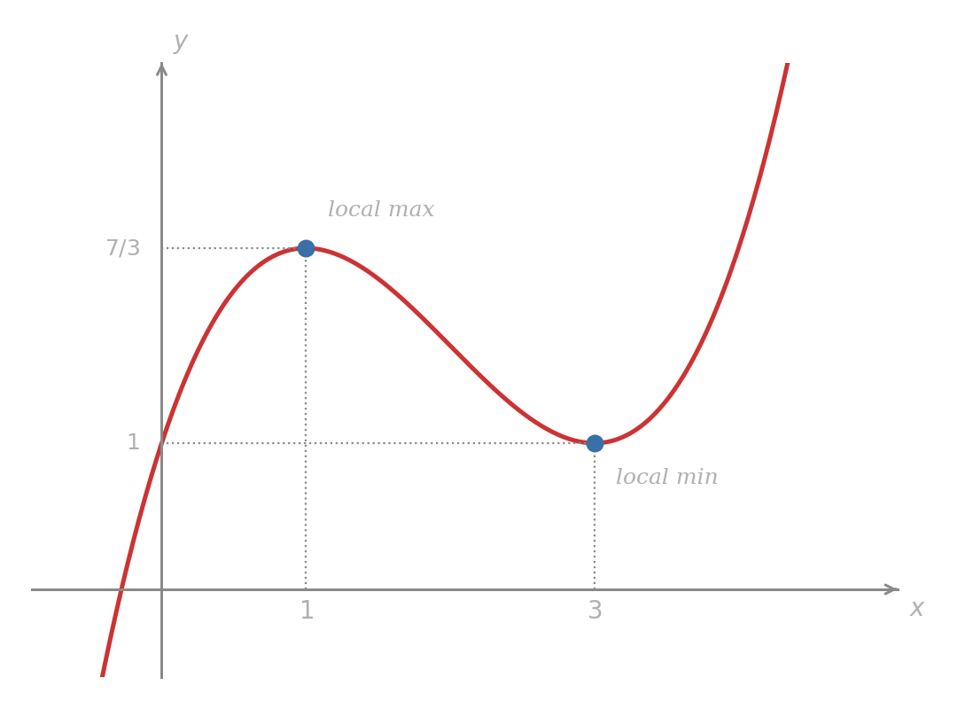
Find the local maximum and minimum points of .
Step 1: find critical numbers. Differentiating,
Setting gives and .
Step 2: evaluate at the critical numbers.
The critical points are and .
Step 3: sign chart. The critical numbers divide the real line into three intervals. Sampling each factor at a representative input from each interval:
| interval | ||||
|---|---|---|---|---|
| increasing | ||||
| local max | ||||
| decreasing | ||||
| local min | ||||
| increasing |
The sign of changes from to at (local maximum) and from to at (local minimum).
Problem 74
Find the local maximum and minimum points of each function, showing a sign chart.
- .
- .
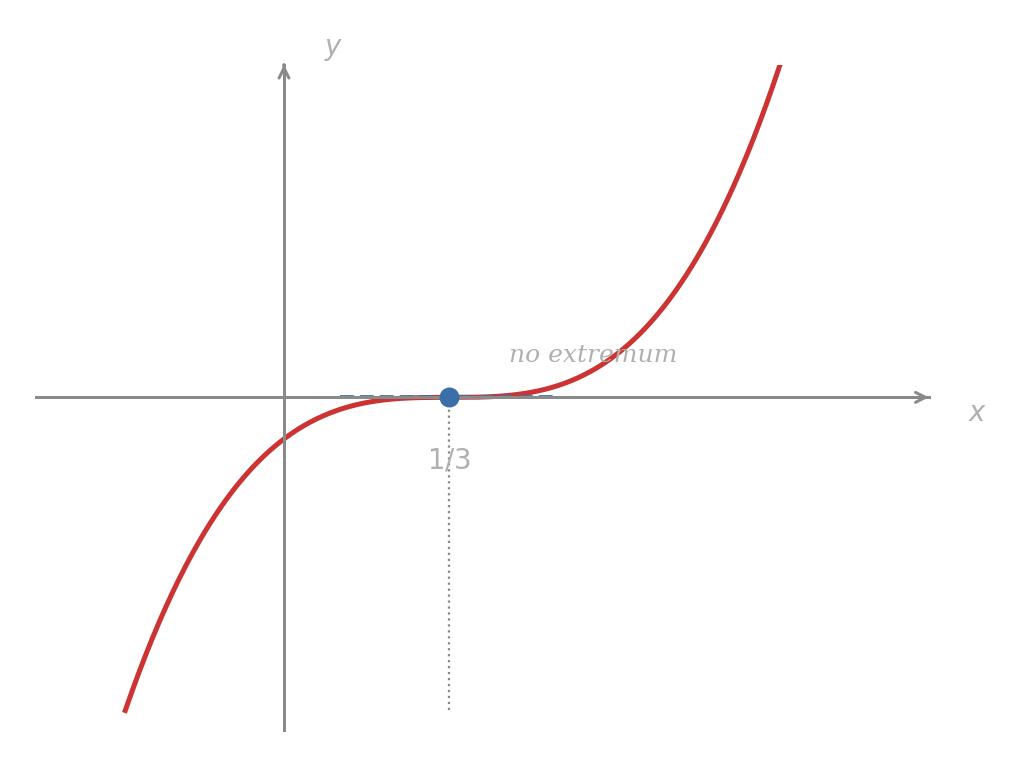
Find the local maximum and minimum points of .
Differentiating by the General power rule from Recitation 2,
Setting gives , so the only critical number is , with .
Since is a perfect square, it is non-negative for all and equals zero only at . So on both sides of : the sign does not change. By case (c) of the first derivative test, there is no local extremum at . The function is increasing on its entire domain; the slope only pauses at zero before continuing upward.
Problem 75
For each function, find all critical numbers, construct a sign chart, and classify each critical point.
- .
- .
After a patient takes a dose, the amount of drug in the bloodstream (in mg) is modelled for the first six hours by
The Real-World Applications section described the shape of this type of curve — rising to a peak, then falling as the body clears the drug. The first derivative test now locates that peak exactly.
Differentiating,
Setting gives and . The value is the left end of the time interval, while is the turning point inside the interval. For , the factor is negative and the factor is negative, so and is increasing. For , the factor is negative and is positive, so and is decreasing. The sign changes from positive to negative at : a local maximum.
The peak concentration is
Problem 76
A market stall owner sets the price of a bowl of soup at pounds. At this price, bowls are sold per day. Write the daily revenue as a function of , locate the critical number, apply the first derivative test, and determine the price that maximises revenue. What is that maximum revenue?
Problem 77
For the drug model above:
- Compute and evaluate it at .
- Use the second derivative rule to determine whether is concave up or concave down at .
- Explain why the sign of confirms that gives a local maximum rather than a local minimum.
The Second Derivative Test
The first derivative test locates extrema by watching the sign of flip across a critical number — a reliable sign chart, but one that requires testing on both sides. When is straightforward to compute, a single evaluation at the critical number is enough.
Return to the drug model from the Peak Drug Concentration example. The sign chart confirmed a local maximum at . We also know , so
Since and , the graph is concave down at — a horizontal tangent sitting atop a downward arch. A local maximum is the only possibility. The sign chart is unnecessary.
Let be a critical number of with .
-
If , then has a local maximum at .
-
If , then has a local minimum at .
-
If , the test is inconclusive: may have a local maximum, a local minimum, or no extremum at .
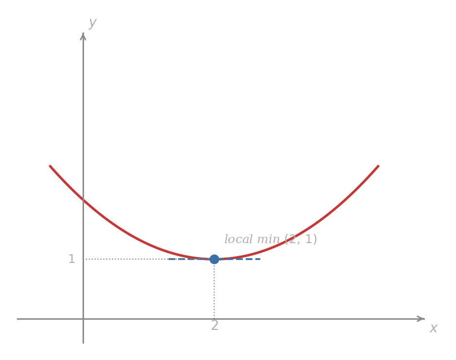
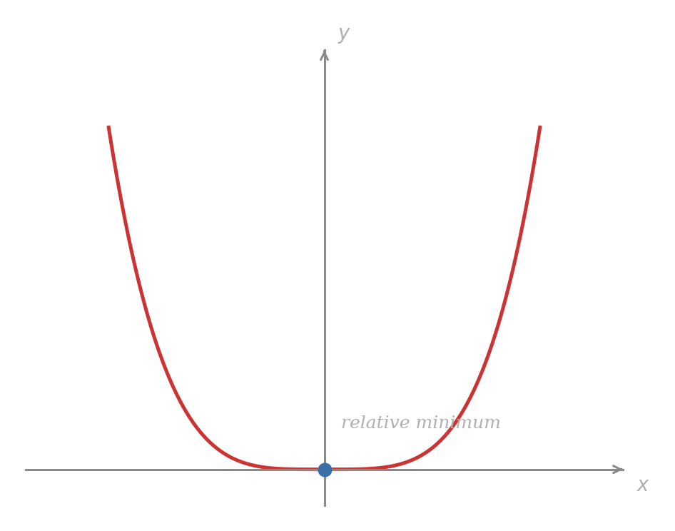
Locate the extreme point of .
Setting gives , the only critical number, with . Since everywhere, the second derivative test gives a local minimum at .
Because is positive everywhere, the graph is concave up throughout; no other critical numbers exist, so this is also the absolute minimum.
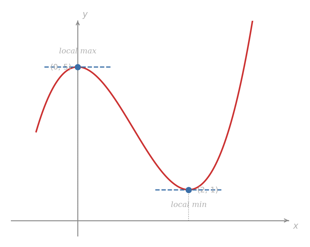
Locate all extreme points of .
The critical numbers are and . Evaluating:
Applying the second derivative test:
Problem 78
Apply the second derivative test to find and classify all extreme points.
- .
- .
Problem 79
In the profit model from the first and second derivative rules problem, you located a critical number using the first derivative rule. Apply the second derivative test to classify it and confirm the same answer.
Locating Inflection Points
The second derivative test classifies the critical points but leaves the shape of the graph between them unresolved. The inflection points from the Inflection Points section fill that gap.
For the cost curve in the Connections section, the inflection at emerged from setting . More generally, candidates for inflection points occur where or where is undefined, provided the original function is continuous there. A concavity check on each side confirms which candidates are genuine inflection points.
Find the inflection point of , and explain why the graph between the two extreme points has exactly one shape transition.
From the previous example, . Setting gives , with .
- For : , so is concave down.
- For : , so is concave up.
The concavity reverses at , confirming an inflection point at .
The second derivative test found a local maximum at (concave down) and a local minimum at (concave up). Since changes sign exactly once — at between these two points — the concavity transitions through and nowhere else. This rules out the “wiggly” alternative sketch that would require additional concavity changes.
Problem 80
Find all inflection points, confirming each is genuine by checking the sign of on both sides.
- .
- .
Problem 81
For the drug model :
- Set and find the inflection point of the concentration curve.
- What does this inflection point say, in practical terms, about how the rate of drug absorption is changing before and after that moment?
A Complete Sketch
With critical points classified and inflection points located, a full sketch follows a three-step sequence.
Step 1. Find the critical numbers: inputs in the domain where or where does not exist. Plot the critical points and classify each using the second derivative test when it applies, or the first derivative test otherwise. If the domain has endpoints, plot and check those separately.
Step 2. Find candidates for inflection points: inputs where or where does not exist. Verify a concavity change at each candidate.
Step 3. Connect the plotted points using the sign of on each interval, and add intercepts and asymptotes from the Summary.
A pop-up market stall runs over six operating days. As the number of promotional hours invested each day grows, the daily revenue (in hundreds of pounds) follows the model
The initial dip reflects setup costs absorbed in early promotion. The three-step procedure locates the turnaround and the peak.
Step 1: Critical points.
Critical numbers: and . Values:
Step 2: Classify.
.
The stall operates at a loss at (revenue is negative), crosses break-even as promotional effort grows, and peaks at .
Step 3: Inflection.
Setting gives . Since and , the concavity reverses at . The inflection point is .
At , the rate of revenue growth transitions from accelerating to decelerating — the stall is still gaining but the gains are shrinking. The full sketch connects all three plotted features.
Problem 82
Apply the three-step procedure to sketch . Identify the local maximum, local minimum, and inflection point. On which interval is the function simultaneously increasing and concave down?
Problem 83
The weekly output of a factory over the first five weeks of a production run is modelled by
From the first and second derivative rules problem earlier in this lesson, you have and . Use the second derivative test to classify the critical point inside the interval, state what happens at the endpoint , locate the inflection point, and explain in words what the inflection point means for the rate of output growth.
When the Second Derivative Test Fails
When , the second derivative test is inconclusive. The functions and both satisfy and , yet they behave oppositely at .
For : the derivative is non-negative everywhere and equals zero only at . The sign of does not change at , so by case (c) of the first derivative test, there is no local extremum. The function is increasing throughout and is an inflection point.
For : the derivative is negative for and positive for . The sign changes from negative to positive at , so by case (b) of the first derivative test, is a local minimum.
Both functions defeat the second derivative test at ; the first derivative test resolves the ambiguity in each case.
When is easy to compute, try the second derivative test first — a single evaluation is faster than a sign chart. Revert to the first derivative test when or when computing is harder than checking the sign of directly. The two tests agree on every conclusion whenever both are decisive.
Problem 84
For each function, attempt the second derivative test. If it fails, use the first derivative test to classify the critical point.
- . (Find all critical numbers, not just .)
- .
Intercepts, Undefined Points, and Asymptotes
The last pieces of a curve sketch come from earlier lessons. Lesson 1AM introduced natural domains and the vertical line test; Lesson 1PM introduced - and -intercepts; Lesson 2PM introduced limits at infinity and their connection with horizontal asymptotes. Here we use those ideas as reminders in the final sketching checklist.
For intercepts, remember that a -intercept occurs at , while an -intercept occurs where . A function can have at most one -intercept, but it may have several -intercepts or none at all.
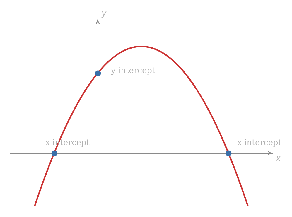
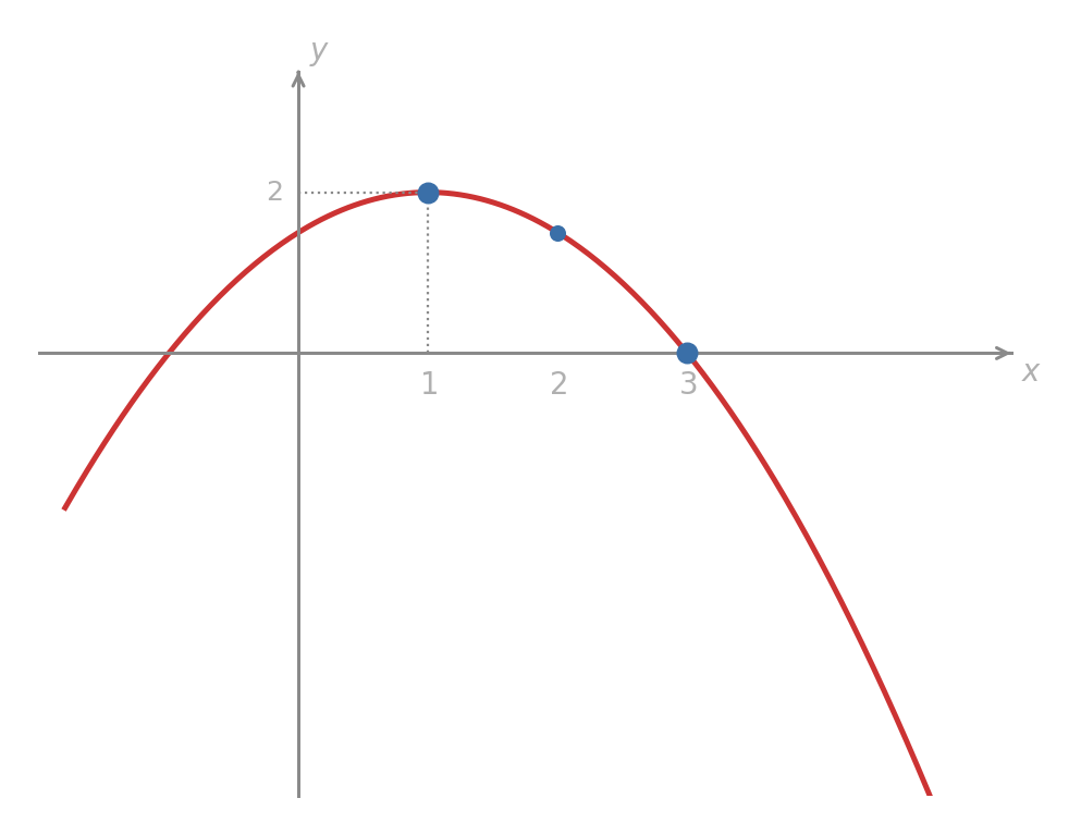
Problem 85
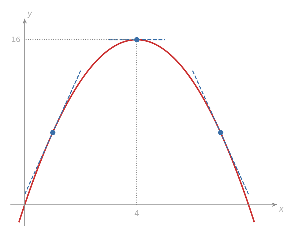
For the displayed parabola , find the intercepts and then add one curve-sketching observation from this lesson: does the graph have a relative maximum or a relative minimum?
Natural-domain restrictions should be carried into the sketch before any other feature is drawn. For instance, a graph of must leave out , while a graph of must leave out . These restrictions were computed in Lesson 1AM; here the point is that a proper sketch must display them.
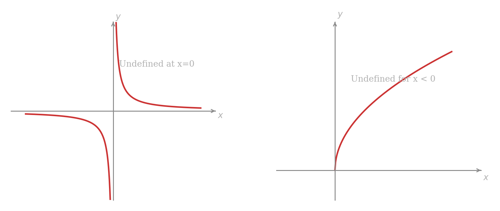
Problem 86
The natural domain of excludes negative inputs and also excludes . When sketching, what two visible features should remind the reader of these restrictions?
Asymptotes record long-run or near-excluded-input behaviour. A horizontal asymptote is read from a limit as or , while a vertical asymptote often appears at an excluded input where function values grow without bound.
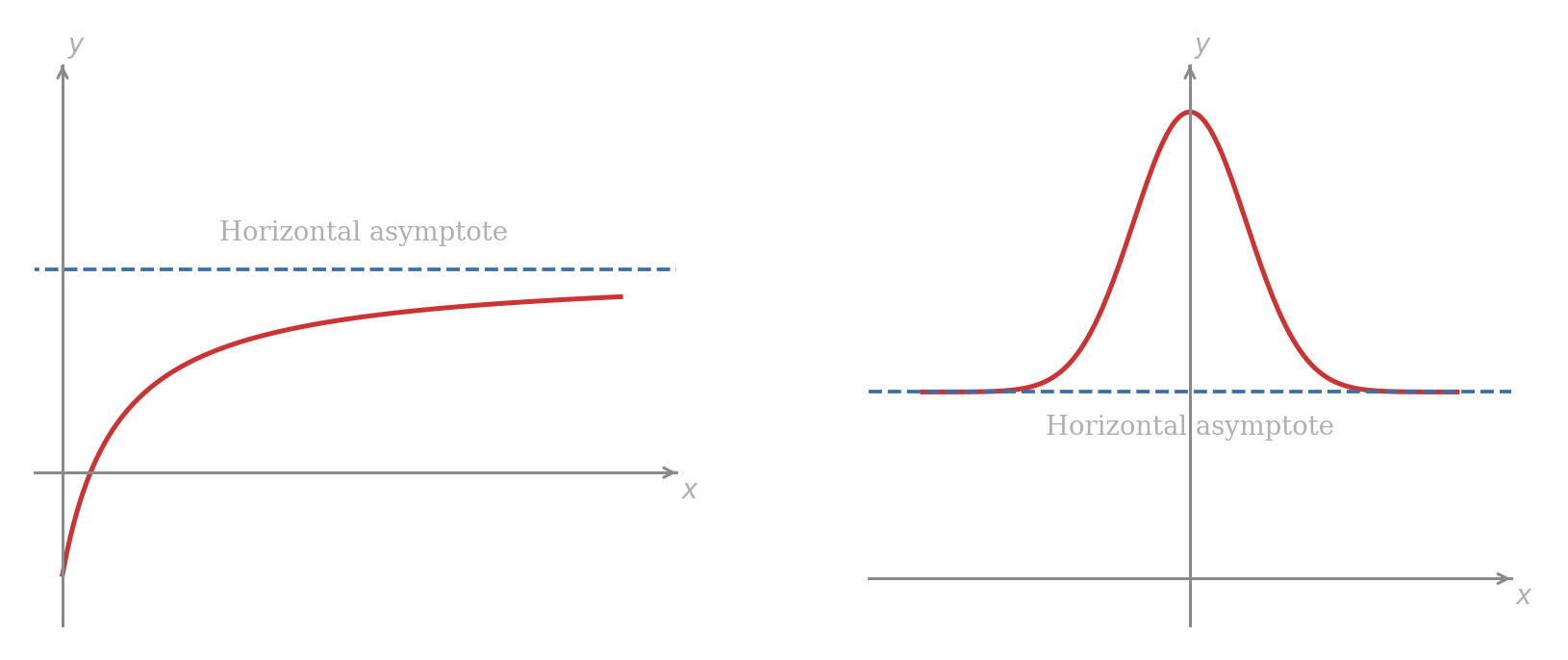
As in Lesson 2PM, if either of the limits
exists, the value of the limit determines a horizontal asymptote.
Problem 87
If , what horizontal asymptote does the graph have to the right? If , what horizontal asymptote does the graph have to the left?
Vertical asymptotes should not be confused with ordinary undefined points. A removable hole leaves out a point; a vertical asymptote describes values that grow without bound as the input approaches the excluded value.
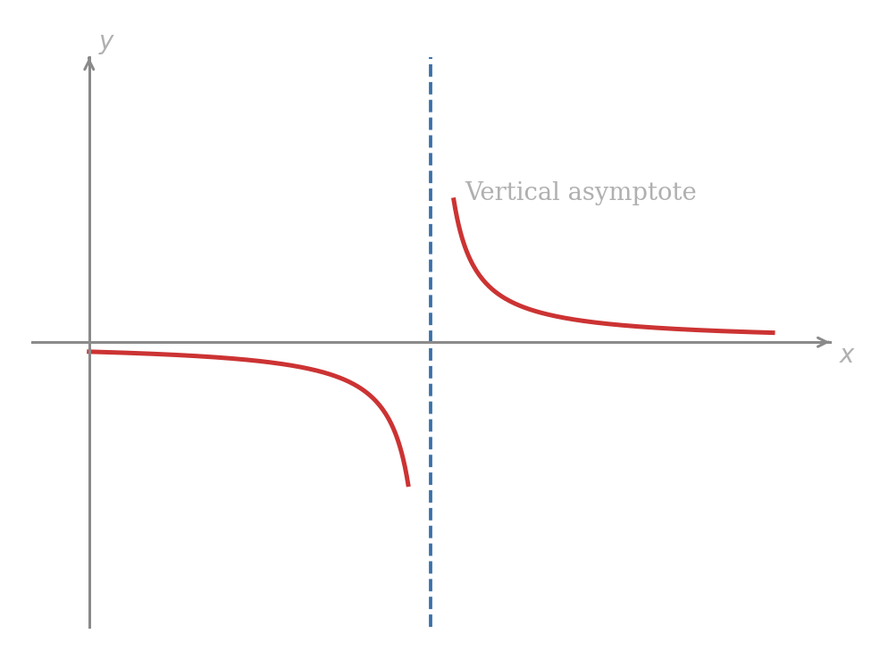
Problem 88
For , where would you expect a vertical asymptote? What horizontal asymptote would you expect as becomes very large in either direction?
Summary of Curve Sketching Properties
We now have six categories for describing the graph of a function:
- Intervals in which the function is increasing (or decreasing), relative maximum points, relative minimum points.
- Maximum value, minimum value.
- Intervals in which the function is concave up (or concave down), inflection points.
- -intercepts, -intercept.
- Undefined points.
- Asymptotes.
For our study of optimisation and derivatives, the first three categories will be the most important. However, the last three categories should never be forgotten when constructing a full, accurate graph.
Problem 89
Describe the graph below. Your description should include each of the six categories listed above, using qualitative language for features whose exact coordinates are not marked.