09/02/2026

#Math#Differentiation

Video

Lesson assets

video link

CS50P Lecture 0: Functions, Variables

exercise

Exercise 1 PDF

Review of Functions

Real Numbers

Differentiation describes how one real-valued quantity responds when another is perturbed, so every object in this course eventually resolves to a real number. Before functions can be discussed honestly, we must agree on what their inputs are and how we describe collections of those inputs.

For the purposes of this course it suffices to regard a real number as an infinite decimal expansion. A rational number is one whose decimal either terminates or eventually repeats; an irrational number is one whose decimal neither terminates nor repeats. Examples are

-\tfrac{5}{2} = -2.5, \qquad \tfrac{13}{3} = 4.333\ldots \qquad \text{(rational)},

\sqrt{2} = 1.414213\ldots, \qquad \pi = 3.14159\ldots \qquad \text{(irrational)}.

The decimal picture carries one ambiguity worth flagging: a real number whose decimal terminates admits a second expansion ending in an infinite string of $9$ s, for instance $1 = 0.999\ldots$ and $-2.5 = -2.4999\ldots$ . Whenever two decimals differ only in this way we treat them as naming the same real number. No other non-uniqueness arises.

A letter such as $x$ is called a real variable when we intend for it to stand for any one real number.

Geometrically, fix an infinite straight line, choose a point on it to mark $0$ , and choose a unit length. Each real number then corresponds to exactly one point on this line, and each point determines exactly one real number.

The real number line with integer ticks from -4 to 4, and the points -5/2 and 13/3 marked

Definition 1 (The Real Number Line)

The infinite line together with its fixed zero and unit length is called the (real) number line. Each point on the number line is identified with a real number, and each real number with a point; we speak of the number $a$ and the point $a$ interchangeably.

Remark

The real numbers can be constructed rigorously from the rationals, but doing so requires machinery beyond the aims of this course. We will treat the real numbers informally throughout and accept their familiar arithmetic and ordering properties without proof.

Inequalities

Once points have positions on the line, comparison becomes a geometric statement. Four symbols express the possible comparisons between two real numbers $x$ and $y$ :

x < y, \qquad x \leq y, \qquad x > y, \qquad x \geq y,

read respectively as ” $x$ is less than $y$ ”, ” $x$ is less than or equal to $y$ ”, ” $x$ is greater than $y$ ”, and ” $x$ is greater than or equal to $y$ ”. Geometrically, $x < y$ means that the point $x$ lies strictly to the left of $y$ on the number line; $x \leq y$ allows equality.

The expression $a < b < c$ is shorthand for the pair of inequalities $a < b$ and $b < c$ . Analogous meanings are given to $a \leq b \leq c$ , $a < b \leq c$ , and $a \leq b < c$ . The three numbers must retain the same relative positions on the line that the inequality signs dictate when read left to right; a string such as $3 < 4 > 1$ is therefore not written, even though each individual comparison is true, because the middle number is not flanked consistently.

Example 1

Each of the following is a valid reading of the number line: $-2 < 0 < \sqrt{2}$ , and $-\tfrac{5}{2} \leq -\tfrac{5}{2} < \tfrac{13}{3}$ . The statement $1 < 3 > 2$ is not used in this course despite both comparisons being true, because the middle term fails to be ordered consistently with the outer ones.

Problem 1

Combine each pair of inequalities into a single chain of the form $a \;\square\; x \;\square\; b$ , using $<$ or $\leq$ in each slot so that the chain says exactly the same thing as the pair.

$x > -3$ and $x \leq 5$ .
$x \geq 0$ and $x < 7$ .
$2 \leq x$ and $x \leq 2$ .

Intervals

Most of the time we will not be working with the whole number line at once, but with a piece of it cut out by one or two inequalities. The pieces we need for this course are exactly the intervals.

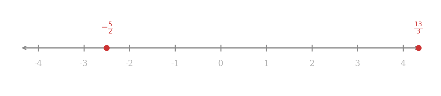
Let $a$ and $b$ be real numbers with $a < b$ . The real numbers $x$ satisfying $a \leq x \leq b$ correspond geometrically to the segment from $a$ to $b$ with both endpoints included. Removing one or both endpoints gives the remaining bounded intervals. When there is no finite upper or lower endpoint, we write $\infty$ or $-\infty$ to indicate that the segment extends without bound; neither symbol denotes a real number.

Definition 2 (Intervals)

Let $a$ and $b$ be real numbers with $a < b$ . The intervals with endpoints $a$ and $b$ are the collections of all real numbers $x$ satisfying the inequality shown in the right-hand column below:

\begin{aligned} [a,b] &\quad\leftrightarrow\quad a \leq x \leq b, \\ (a,b) &\quad\leftrightarrow\quad a < x < b, \\ [a,b) &\quad\leftrightarrow\quad a \leq x < b, \\ (a,b] &\quad\leftrightarrow\quad a < x \leq b. \end{aligned}

The intervals with only one finite endpoint are

\begin{aligned} [a,\infty) &\quad\leftrightarrow\quad x \geq a, & (a,\infty) &\quad\leftrightarrow\quad x > a, \\ (-\infty, b] &\quad\leftrightarrow\quad x \leq b, & (-\infty, b) &\quad\leftrightarrow\quad x < b. \end{aligned}

The interval $[a,b]$ is called closed; $(a,b)$ is called open. An interval is half-open if exactly one endpoint is included.

Remark

The symbols $\infty$ and $-\infty$ mark that the interval is unbounded above or below. An inequality describing an unbounded interval may be written in two equivalent ways: $a < x$ and $x > a$ describe the same interval $(a, \infty)$ .

Graphically, a bounded interval is drawn as the segment of the number line between its endpoints, with a filled circle at an included endpoint and an unfilled circle at an excluded one. An unbounded interval is drawn with an arrow in place of the missing endpoint.

Four line segments illustrating intervals (a) (-1, 2) with open endpoints, (b) [-2, 7] with closed endpoints, (c) (2, infinity) with an open left endpoint, (d) (-infinity, sqrt(2)] with a closed right endpoint

Example 2

The four intervals shown above each illustrate one of the endpoint conventions.

$(-1, 2)$ consists of every real $x$ with $-1 < x < 2$ ; both endpoints are excluded, shown as unfilled circles.
$[-2, 7]$ consists of every real $x$ with $-2 \leq x \leq 7$ ; both endpoints are included, shown as filled circles.
$(2, \infty)$ consists of every real $x$ with $x > 2$ ; the segment extends without bound to the right, so the right end of the drawing is an arrow rather than a circle.
$(-\infty, \sqrt{2}\,]$ consists of every real $x$ with $x \leq \sqrt{2}$ ; the left end is unbounded, the right endpoint is included.

Example 3

A machine shop can only operate its lathe at positive rotational speeds, and safety limits cap the speed at $3000$ revolutions per minute. Writing $\omega$ for the speed, the admissible values form the half-open interval $(0, 3000]$ : zero is excluded because the machine is then idle, while $3000$ is included as the highest safe setting.

Problem 2

Describe each of the following as an interval and sketch it on the number line.

All real $x$ satisfying $-1 \leq x < 4$ .
All real $x$ satisfying $x^2 < 9$ .
All real $x$ satisfying $x \geq -\pi$ .
All real $x$ that are both strictly greater than $-2$ and less than or equal to $\sqrt{2}$ .

Problem 3

A reservoir has capacity $500$ cubic metres and cannot hold a negative volume. Let $V$ denote the volume of water in the reservoir at a given time. Express the physically meaningful values of $V$ as an interval, and state whether each endpoint is open or closed.

The reason for dwelling on intervals is that they are exactly the collections of inputs we will hand to formulas later in this course.

Example 4

The expression $\sqrt{x}$ produces a real number precisely when $x \geq 0$ , so the admissible inputs form the unbounded interval $[0, \infty)$ . The expression $\sqrt{1 - x}$ requires $1 - x \geq 0$ , that is $x \leq 1$ , and its admissible inputs form $(-\infty, 1]$ . In each case the admissible inputs are described entirely by an interval. Intervals, sometimes with a few points removed, will supply the inputs for every formula we meet.

Problem 4

Determine all real $x$ for which the expression $\sqrt{x - 2} + \sqrt{5 - x}$ is defined, and write the answer as an interval.

Example 5

Given a fixed real number $a$ and a positive real number $\delta$ , every $x$ satisfying $a - \delta < x < a + \delta$ lies in the open interval $(a - \delta, a + \delta)$ , and conversely. When we later say ” $x$ is close to $a$ ”, we will mean $x$ lies in an interval of this form for some (possibly small) $\delta$ .

Functions

Differentiation is a study of how one numerical quantity responds to changes in another. Before we can track how a quantity responds, we must agree on what it means for one quantity to be determined by another at all. The honest answer is the idea of a function.

A prototype is the formula $y = x^2$ . For each real variable $x$ , the formula produces exactly one real number $y$ , namely the square of $x$ . Two people handed the same $x$ must arrive at the same $y$ . This single-valuedness is what distinguishes a function from a looser kind of correspondence.

Definition 3 (Function)

A function $f$ is a rule that assigns to each real variable $x$ drawn from a prescribed collection of inputs exactly one real number, denoted $f(x)$ and read ” $f$ of $x$ ”. The number $f(x)$ is the value of $f$ at $x$ .

The collection of admissible inputs is the domain of $f$ ; the collection of all values $f(x)$ produced as $x$ runs over the domain is the range of $f$ . The letter $x$ is the independent variable. When we write $y = f(x)$ , the letter $y$ is the dependent variable, its value being fixed as soon as $x$ is chosen.

Remark

A formula is one way to specify a rule, but not the only one. Any unambiguous prescription that produces a single real number from each admissible input qualifies as a function. In this course every function will ultimately be described by one or more formulas, but the definition itself is formula-free.

Example 6

Let $p(x) = 2x^3 - 5x^2 + x + 4$ . Substituting $x = 3$ ,

p(3) = 2 \cdot 27 - 5 \cdot 9 + 3 + 4 = 54 - 45 + 3 + 4 = 16,

and substituting $x = -1$ ,

p(-1) = 2(-1) - 5(1) + (-1) + 4 = -2 - 5 - 1 + 4 = -4.

Polynomial evaluation requires only addition and multiplication of real numbers, so every real $x$ is admissible: the domain of $p$ is the whole number line.

Problem 5

Let $f(x) = x^3 - 3x$ . Compute $f(0)$ , $f(5)$ , $f(3)$ , and $f(-7)$ .

Building new functions from old

The argument of a function need not be a bare letter. Any expression whose own value is a real number may be substituted, provided the resulting input still lies in the domain. Most functions in this course will be assembled this way: from a handful of basic rules, combined by evaluating one inside another.

Example 7

The area of a disc of radius $r \geq 0$ is $A(r) = \pi r^2$ . The area added when the radius increases from $r$ to $r + 1$ is

g(r) = A(r + 1) - A(r) = \pi (r + 1)^2 - \pi r^2 = \pi (2r + 1).

Here $g$ is assembled from $A$ by evaluation at $r + 1$ and at $r$ and subtraction. Its admissible inputs are the same as those of $A$ , namely $r \geq 0$ , and $g(r)$ is the area gained when the radius grows from $r$ to $r + 1$ .

Example 8

Let $f(x) = \dfrac{4 - x}{x^2 + 3}$ . At an arbitrary real $a$ ,

f(a) = \frac{4 - a}{a^2 + 3},

and at $a + 1$ ,

f(a + 1) = \frac{4 - (a + 1)}{(a + 1)^2 + 3} = \frac{3 - a}{a^2 + 2a + 4}.

The denominator $x^2 + 3$ is never zero, so every real $x$ is admissible.

Problem 6

Let $f(x) = \dfrac{1}{x - 2}$ . Write $f(a)$ and $f(a + h)$ , and simplify the difference $f(a + h) - f(a)$ over a common denominator. State the admissible inputs of $f$ .

Graphs

A formula can be drawn. Take two perpendicular copies of the number line sharing a common zero, one horizontal and called the $x$ -axis, one vertical and called the $y$ -axis. The resulting plane, equipped with these two axes, is the $xy$ -plane. Each ordered pair of real numbers $(x, y)$ then marks a unique point of the $xy$ -plane, with $x$ read off the horizontal axis and $y$ off the vertical.

Definition 4 (Graph of a Function)

The graph of a function $f$ is the collection of points $(x, f(x))$ obtained as $x$ runs over the domain of $f$ . The horizontal axis records the independent variable $x$ ; the vertical axis records the dependent variable $y = f(x)$ .

The graph of y = x squared, drawn as a parabola through the origin, with the point (2, 4) marked and dashed lines dropped to each axis

Example 9

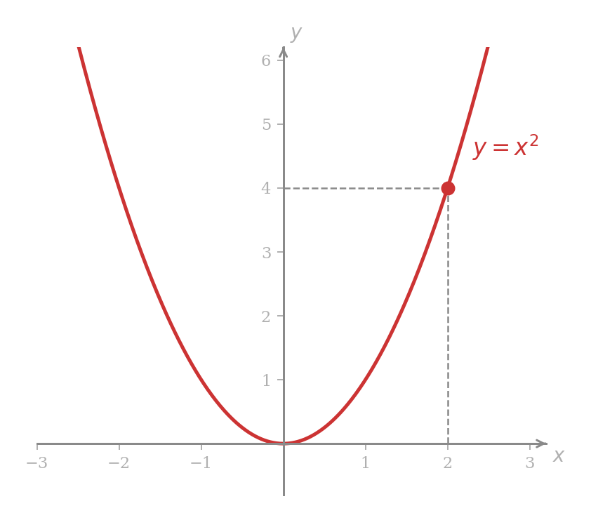
The graph of $y = x^2$ is a parabola opening upward. At $x = 2$ the height is $y = 4$ , giving the point $(2, 4)$ shown above. Every real $x$ produces a real $y$ , so the admissible inputs cover the whole horizontal axis; because $x^2 \geq 0$ always, the range is $[0, \infty)$ .

Sketching by plotting points

A graph can be approximated directly from a formula by evaluating $f$ at a representative spread of inputs, plotting the resulting points, and joining them by a smooth curve. The more closely spaced the inputs, the closer the approximation.

Example 10

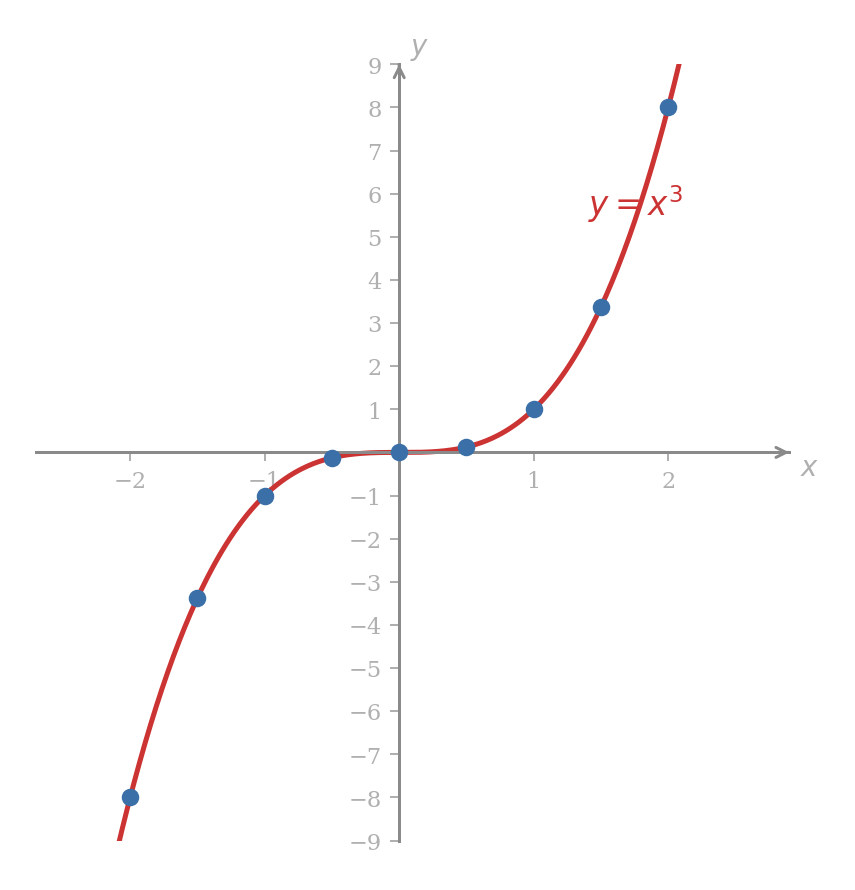
Sketch the graph of $f(x) = x^3$ .

Cubing is defined for every real number, so every real $x$ is admissible. Tabulating at evenly spaced inputs gives

$x$	$-2$	$-1.5$	$-1$	$-0.5$	$0$	$0.5$	$1$	$1.5$	$2$
$f(x)$	$-8$	$-3.375$	$-1$	$-0.125$	$0$	$0.125$	$1$	$3.375$	$8$

Plotting these nine points and joining them by a smooth curve produces the graph shown below. The curve climbs steeply for $|x|$ large, and is almost flat near the origin, as the table already suggests.

The graph of y = x cubed passing through the origin, with nine marked sample points at x = -2, -1.5, -1, -0.5, 0, 0.5, 1, 1.5, 2; the curve rises steeply on the right and falls steeply on the left

When the admissible inputs exclude a point, the behaviour of $f$ near that point is often the most interesting part of the sketch, so the tabulation should include inputs approaching the forbidden point from both sides.

Example 11

Sketch the graph of $f(x) = \dfrac{1}{x}$ .

The formula is defined for every real $x$ except $x = 0$ . Tabulating on either side of the excluded point,

$x$	$-3$	$-2$	$-1$	$-\tfrac{1}{2}$	$\tfrac{1}{2}$	$1$	$2$	$3$
$f(x)$	$-\tfrac{1}{3}$	$-\tfrac{1}{2}$	$-1$	$-2$	$2$	$1$	$\tfrac{1}{2}$	$\tfrac{1}{3}$

shows that the values grow without bound as $x$ approaches $0$ from the right, and fall without bound as $x$ approaches $0$ from the left. The graph therefore splits into two branches, one for $x < 0$ and one for $x > 0$ , neither of which crosses the vertical axis.

The graph of y = 1/x in two disconnected branches: one in the third quadrant for x < 0 and one in the first quadrant for x > 0, with marked sample points on each branch; neither branch meets the vertical axis

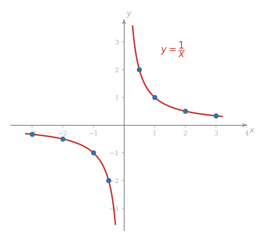
The admissible inputs of $f(x) = 1/x$ illustrate a phenomenon absent from the previous examples: they are not a single interval but two disconnected pieces, one strictly to the left of $0$ and one strictly to the right. We will return to this point in the section on natural domains.

Linear functions

Amongst the simplest graphs are those of linear functions. They will serve throughout the course as the local model for more complicated graphs: zoomed in far enough, the graph of a well-behaved function looks straight, and the derivative will be the slope of that straight line.

Definition 5 (Linear Function)

A linear function is a function of the form $f(x) = mx + b$ , where $m$ and $b$ are fixed real numbers. Its graph is a straight line. The number $m$ is the slope of the line, and $b$ is its $y$ -intercept, the value $f(0)$ at which the line crosses the vertical axis.

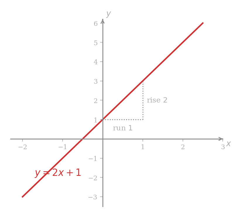
The line y = 2x + 1, with a dotted right-triangle showing that a run of 1 to the right produces a rise of 2 upward, illustrating slope 2

Geometrically, the slope $m$ records how much $y$ changes for each unit change in $x$ : increasing $x$ by $1$ increases $y$ by exactly $m$ . In the figure, $y = 2x + 1$ rises by $2$ for each unit step to the right, so the dotted rise-over-run triangle has slope $2$ , and the line meets the $y$ -axis at $1$ .

Vertical and horizontal shifts

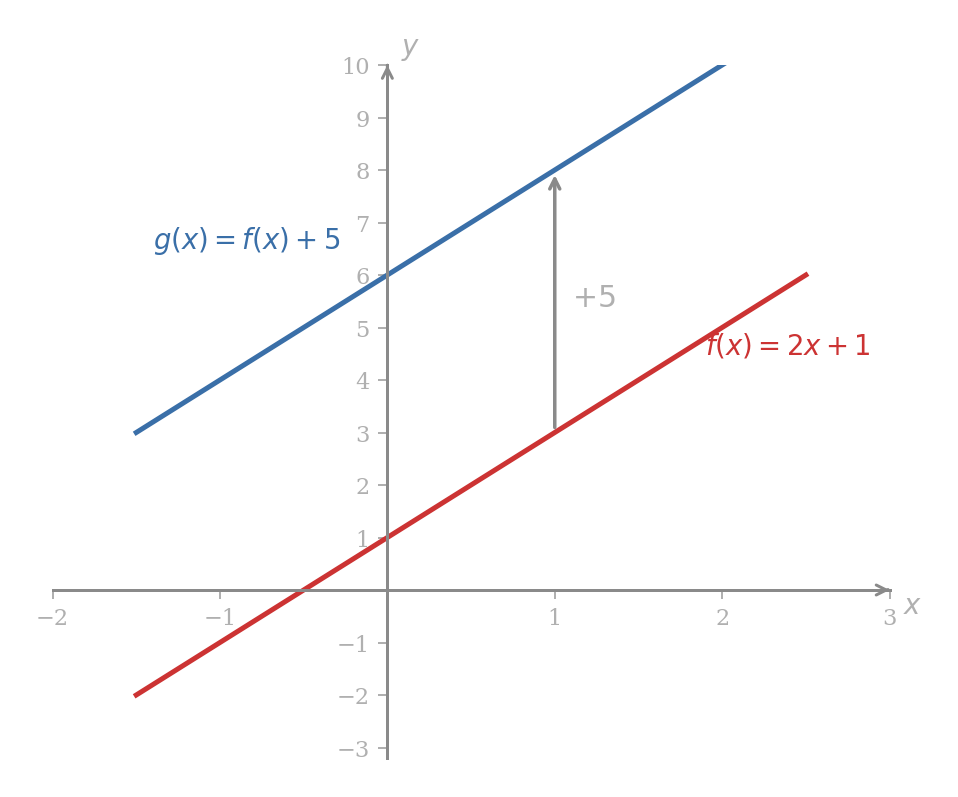
Given any function $f$ , certain simple modifications of its formula move the graph bodily without deforming it. The next two constructions are worth isolating because the local approximation story later in the course will repeatedly use shifted copies of the same line.

Example 12

Let $f(x) = 2x + 1$ and set $g(x) = f(x) + 5 = 2x + 6$ . At every $x$ the value of $g$ exceeds the value of $f$ by exactly $5$ , so the graph of $g$ is obtained from the graph of $f$ by sliding every point upward by $5$ units.

Two parallel lines with the same slope: the lower line is y = 2x + 1 and the upper line is y = 2x + 6, related by a vertical upward shift of 5 units

Example 13

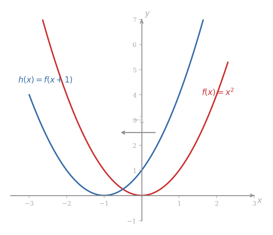
Let $f(x) = x^2$ and set $h(x) = f(x + 1) = (x + 1)^2$ . The value of $h$ at $x$ is the value of $f$ at $x + 1$ , so whatever $f$ does one unit to the right, $h$ does at $x$ itself. The graph of $h$ is the graph of $f$ slid one unit to the left.

Two parabolas of the same shape: y = x squared centred at the origin, and y = (x+1) squared centred at x = -1, related by a horizontal leftward shift of 1 unit

More generally, for a real number $c$ :

$f(x) + c$ shifts the graph vertically, upward by $c$ when $c > 0$ and downward by $|c|$ when $c < 0$ ;
$f(x + c)$ shifts the graph horizontally, leftward by $c$ when $c > 0$ and rightward by $|c|$ when $c < 0$ .

The sign on the horizontal shift is easy to misremember. The rule is that replacing $x$ by $x + c$ reaches the former output when $x$ is $c$ smaller than before, pulling the graph back along the $x$ -axis.

Piecewise functions

Nothing in the definition of a function requires a single formula. When different parts of the domain call for different rules, we write the rule piece by piece.

Example 14

Define

f(x) = \begin{cases} -x, & x \leq 1, \\ x^2, & x > 1. \end{cases}

For $x = 0$ the top clause applies and $f(0) = 0$ . For $x = 2$ the bottom clause applies and $f(2) = 4$ . At the switchover $x = 1$ only the top clause applies, so $f(1) = -1$ ; the bottom clause’s value $1^2 = 1$ is never attained at $x = 1$ itself.

A piecewise graph: the line y = -x for x less than or equal to 1, joined at x = 1 with a filled circle at (1, -1), and the parabola y = x squared for x greater than 1 with an unfilled circle at (1, 1)

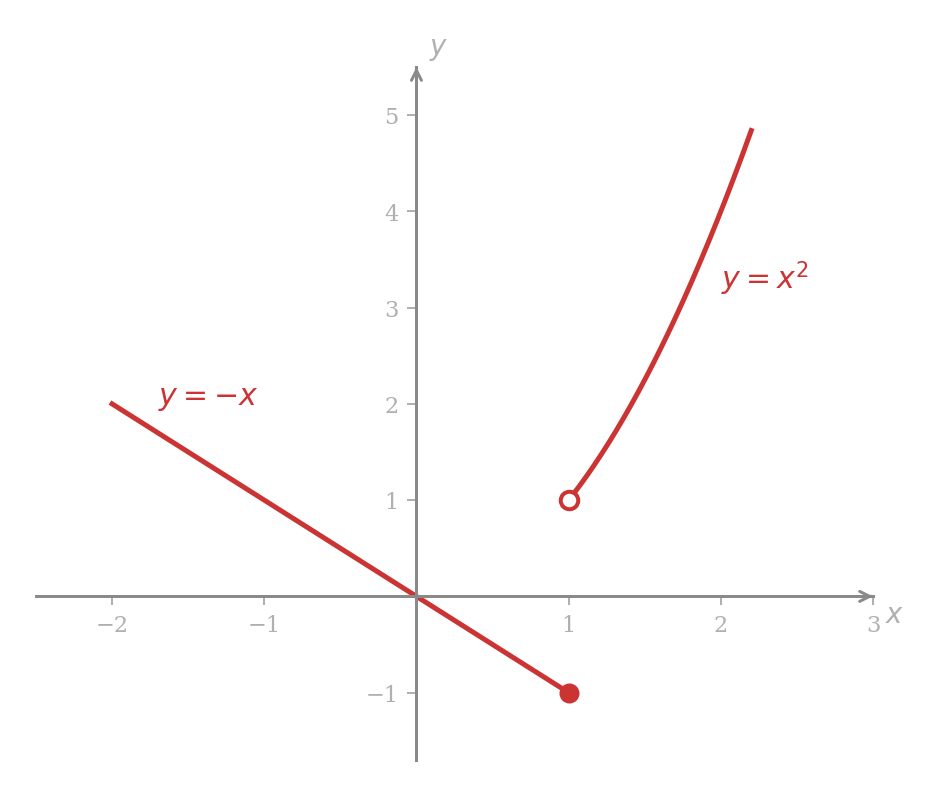
The graph uses the filled and unfilled circle convention already established for intervals. At $x = 1$ the top clause contributes the point $(1, -1)$ , drawn with a filled circle because the value is actually attained; the bottom clause approaches $(1, 1)$ without reaching it, drawn with an unfilled circle.

Example 15

A parcel courier posts the following tariff. A parcel of weight $w$ kilograms, with $0 < w \leq 2$ , is charged a flat $\pounds 4.00$ . A heavier parcel with $w > 2$ is charged $\pounds 4.00$ plus $\pounds 1.20$ for each kilogram beyond the first two. Writing the charge $C$ as a function of weight,

C(w) = \begin{cases} 4.00, & 0 < w \leq 2, \\ 4.00 + 1.20\,(w - 2), & w > 2. \end{cases}

Thus a $1.5$ kg parcel is charged $\pounds 4.00$ , a $3$ kg parcel $\pounds 5.20$ , and a $5$ kg parcel $\pounds 7.60$ . The domain is the positive half-line $(0, \infty)$ , since a parcel must have some strictly positive weight.

Problem 7

The courier of the previous example revises the tariff by adding a third tier: for any parcel with $w > 10$ , the charge is what the middle tier would have cost at exactly $10$ kg, plus $\pounds 0.80$ for each kilogram beyond the first ten. Write the revised charge $C(w)$ as a piecewise function on $(0, \infty)$ and compute $C(7)$ and $C(14)$ .

Natural Domains

In the examples so far we have either stated a function’s admissible inputs alongside its formula or read them off the formula by inspection. From now on we will usually present a function by writing a formula and nothing else, and leave the inputs to be recovered from the formula itself. The convention for doing so is the following.

Definition 6 (Natural Domain)

When a function is specified by a formula with no domain attached, its natural domain is the collection of all real numbers for which every operation in the formula produces a real result.

For the formulas considered in this lesson, only two obstructions can arise: division by zero, and the square root of a negative number. (Later lessons will introduce further functions, such as logarithms and certain trigonometric functions, which bring their own restrictions; we will record these as each new function is introduced.) Each obstruction rules out a definite collection of inputs, and the natural domain is determined by imposing whichever conditions are needed to avoid them.

Example 16

The formula $f(x) = x^2 - x + 1$ requires only addition, subtraction, and multiplication, each of which is defined for every real number. No input is obstructed, so the natural domain of $f$ is the whole number line.

Example 17

The formula $g(x) = \dfrac{1}{x}$ is defined whenever $x \neq 0$ , since division by zero is not permitted. The natural domain of $g$ therefore consists of every real $x$ with $x \neq 0$ .

Example 18

The formula $h(x) = \sqrt{x}$ requires the expression under the square root, called the radicand, to be non-negative, giving the condition $x \geq 0$ . The natural domain of $h$ is the interval $[0, \infty)$ .

These three templates each illustrate one obstruction in isolation. Most formulas combine them, and the natural domain is then determined by imposing all of the resulting conditions simultaneously.

Example 19

Find the natural domain of each of the following.

(a) $f(x) = \sqrt{4 + 2x}$ .

The radicand must satisfy $4 + 2x \geq 0$ , that is $x \geq -2$ . The natural domain is $[-2, \infty)$ .

(b) $g(x) = \dfrac{1}{\sqrt{2x + 1}}$ .

Two conditions apply: the radicand must be non-negative and the denominator must be non-zero. Both are satisfied precisely when $2x + 1 > 0$ , equivalently $x > -\tfrac{1}{2}$ . The natural domain is $(-\tfrac{1}{2}, \infty)$ .

(c) $h(x) = \sqrt{x + 1} - \sqrt{1 - x}$ .

Both radicands must be non-negative: $x + 1 \geq 0$ and $1 - x \geq 0$ . The first gives $x \geq -1$ , the second gives $x \leq 1$ . Both conditions must hold, so the natural domain is the closed interval $[-1, 1]$ .

Not every natural domain is a single interval. The following is the cleanest example.

Example 20

Find the natural domain of $f(x) = \dfrac{1}{x^2 - 1}$ .

The numerator is defined for every real $x$ , so the only obstruction is the vanishing of the denominator. Factoring $x^2 - 1 = (x - 1)(x + 1)$ , the denominator is zero precisely when $x = 1$ or $x = -1$ , and every other real $x$ is admissible. The natural domain therefore consists of every real $x$ with $x \neq 1$ and $x \neq -1$ . The two excluded points split this collection into three unbounded pieces:

x < -1, \qquad -1 < x < 1, \qquad x > 1,

each of which is itself an interval. The two excluded points behave in the same way as the excluded point $x = 0$ did for $f(x) = 1/x$ : near each of them the values of $f$ grow without bound in magnitude.

Problem 8

Find the natural domain of $f(x) = \dfrac{3x - 5}{x^2 + x - 6}$ .

Problem 9

Find the natural domain of $f(x) = \sqrt{2x + 7} + \sqrt{x}$ .

Reading Graphs

A great deal of a function’s data can be read directly off its graph, without recourse to any formula.

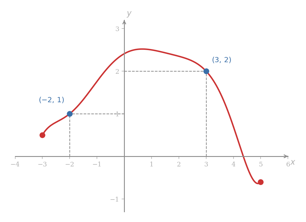
The graph of a smooth function on the domain from -3 to 5; the curve begins near height 0.5 on the left, rises to about 2.5 near x = 1, and falls to about -0.6 at x = 5, with the points (-2, 1) and (3, 2) marked and dashed lines dropped from each marked point to both axes

Example 21

Let $f$ be the function whose graph is shown above.

(a) The point $(3, 2)$ lies on the graph, so $f(3) = 2$ .

(b) The point on the graph at $x = -2$ has height $1$ , so $f(-2) = 1$ .

(c) The graph runs horizontally from $x = -3$ to $x = 5$ , so the domain of $f$ is $[-3, 5]$ . Reading off the heights attained, $f$ takes every value between roughly $-0.6$ at the right endpoint and about $2.5$ near $x = 1$ , so the range of $f$ is approximately $[-0.6,\, 2.5]$ .

Problem 10

Using the graph of $f$ above, answer the following.

Estimate the $x$ -values at which $f(x) = 0$ .
For which $x$ in the domain is $f(x) \geq 2$ ?
Is $f(4)$ positive, negative, or zero? What about $f(5)$ ?
Estimate the value of $f(0)$ .

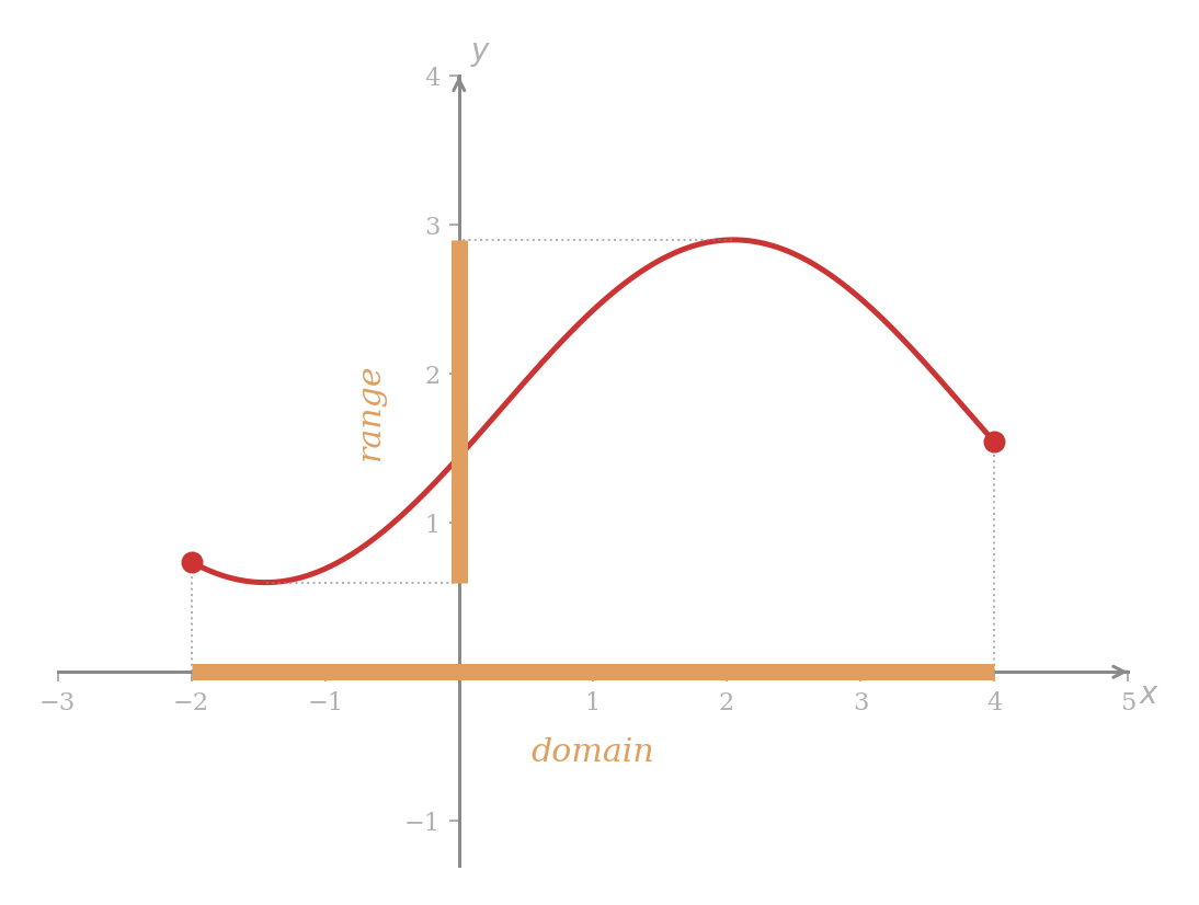
Two conventions are at work in the picture. The domain is read off the horizontal axis as the shadow of the graph projected downward onto it, and the range is read off the vertical axis as the shadow projected sideways. The general situation is illustrated below: the thick amber segment on the horizontal axis is the domain of $f$ , and the thick amber segment on the vertical axis is its range.

A smooth curve on the domain -2 to 4, with its domain drawn as a thick segment on the horizontal axis labelled 'domain', and its range drawn as a thick segment on the vertical axis labelled 'range'; dotted projection lines connect the endpoints and extrema of the curve to each shadow

The vertical line test

Not every curve drawn in the $xy$ -plane is the graph of a function. The definition of a function requires each admissible input to yield exactly one output; two points on the curve with the same $x$ -coordinate but different $y$ -coordinates would mean two candidate outputs at a single input. This geometric failure is easy to detect by eye.

Definition 7 (Vertical Line Test)

A curve in the $xy$ -plane is the graph of a function of $x$ if and only if every vertical line meets the curve in at most one point.

The test is a pictorial restatement of single-valuedness, not a new condition. A vertical line at a chosen $x$ -value meets the curve exactly where that $x$ has a corresponding point on the curve, so at most one meeting corresponds to at most one output.

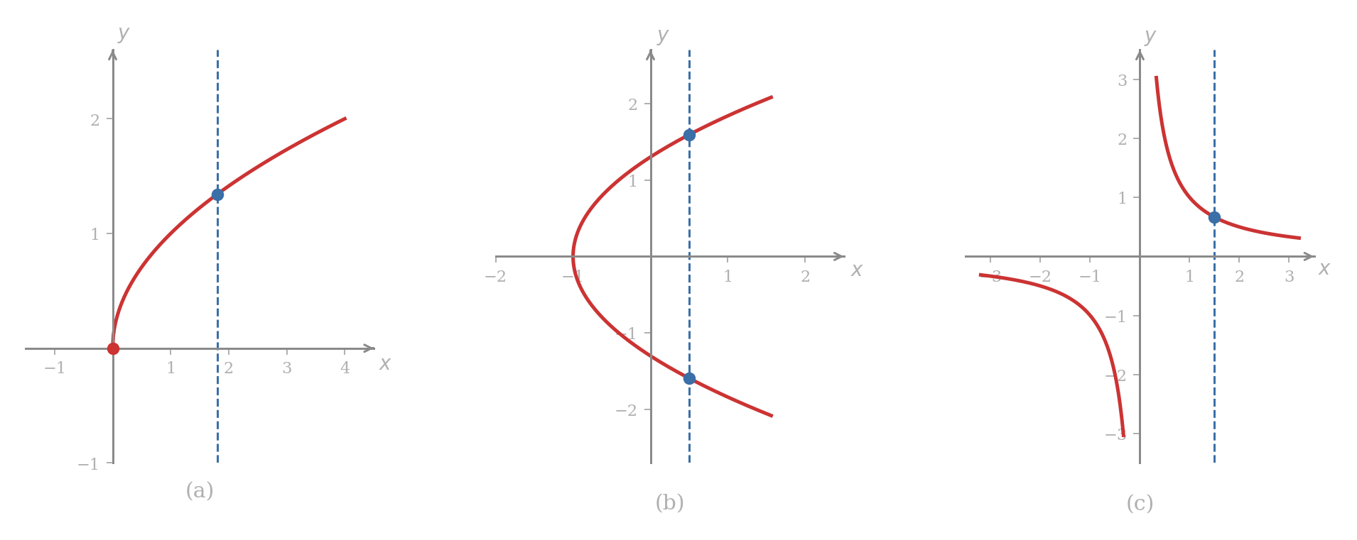
Three curves in the xy-plane, each tested by a dashed vertical line: (a) the graph of y = sqrt(x) for x greater than or equal to 0, which the test line meets in exactly one point; (b) a sideways parabola opening to the right, which the test line meets in two points and therefore fails the test; (c) the two branches of y = 1/x, with the test line meeting only the right branch in exactly one point

Example 22

Each panel above shows a curve and a dashed vertical test line.

(a) Every vertical line to the right of the vertical axis meets the curve once, and vertical lines to the left of the axis do not meet it at all. The curve therefore passes the test; the gap on the left simply reflects that the underlying function is defined only for $x \geq 0$ .

(b) The dashed line meets the curve in two points, so single-valuedness fails. The curve is not the graph of any function of $x$ .

(c) Every vertical line with $x \neq 0$ meets the curve in exactly one point; the vertical axis itself misses the curve entirely, reflecting that the underlying function $f(x) = 1/x$ is not defined at $x = 0$ . The curve therefore passes the test.

Remark

It is common practice to speak of “the function $y = f(x)$ ”, taking $y$ as a stand-in for the values of $f$ . Under this convention, the graph of $f$ and the graph of the equation $y = f(x)$ refer to the same collection of points, and we shall use the two phrasings interchangeably.