09/02/2026

#Math#Differentiation

Video

Lesson assets

alternate video

Alternate video: freeCodeCamp Python basics

A longer outside walkthrough if you want the same foundations taught with a different pacing and style.

recitation

Recitation

Homework 1 PDF

Review of Functions, Continued

Lines in the Plane

The AM lesson introduced a straight line through its slope-intercept formula $y = mx + b$ and, as an instance of the Linear Function definition, the graph was read off directly. That formula misses one family of lines, the perfectly vertical ones, and until we put them back we cannot say cleanly which equations in two variables describe graphs of functions and which do not. Since the lessons ahead will hand us a line at every point where a function has a derivative, it is worth settling the picture now.

Every line in the $xy$ -plane satisfies an equation of the form

c x + d y = e,

where $c$ , $d$ , $e$ are real constants and $c$ and $d$ are not both zero. When $d \neq 0$ , we may divide by $d$ and solve for $y$ ,

y = m x + b, \qquad m = -\frac{c}{d}, \quad b = \frac{e}{d},

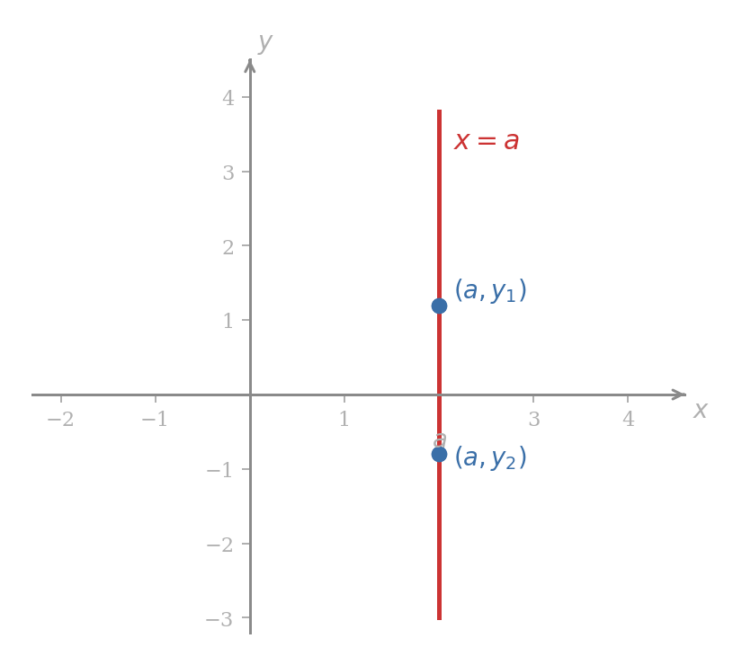
so the line is the graph of the linear function already named in the AM lesson. When $d = 0$ , the equation collapses to $cx = e$ ; since $c$ is then non-zero, dividing by it gives $x = a$ with $a = e/c$ . This last equation picks out every point whose $x$ -coordinate equals $a$ , and so traces the vertical line through $(a, 0)$ .

A vertical line meets itself at every point on it, in particular at all heights above $x = a$ . The vertical line test of the AM lesson then rules at once that $x = a$ is the graph of no function of $x$ : a single input would have to carry infinitely many outputs, contradicting single-valuedness.

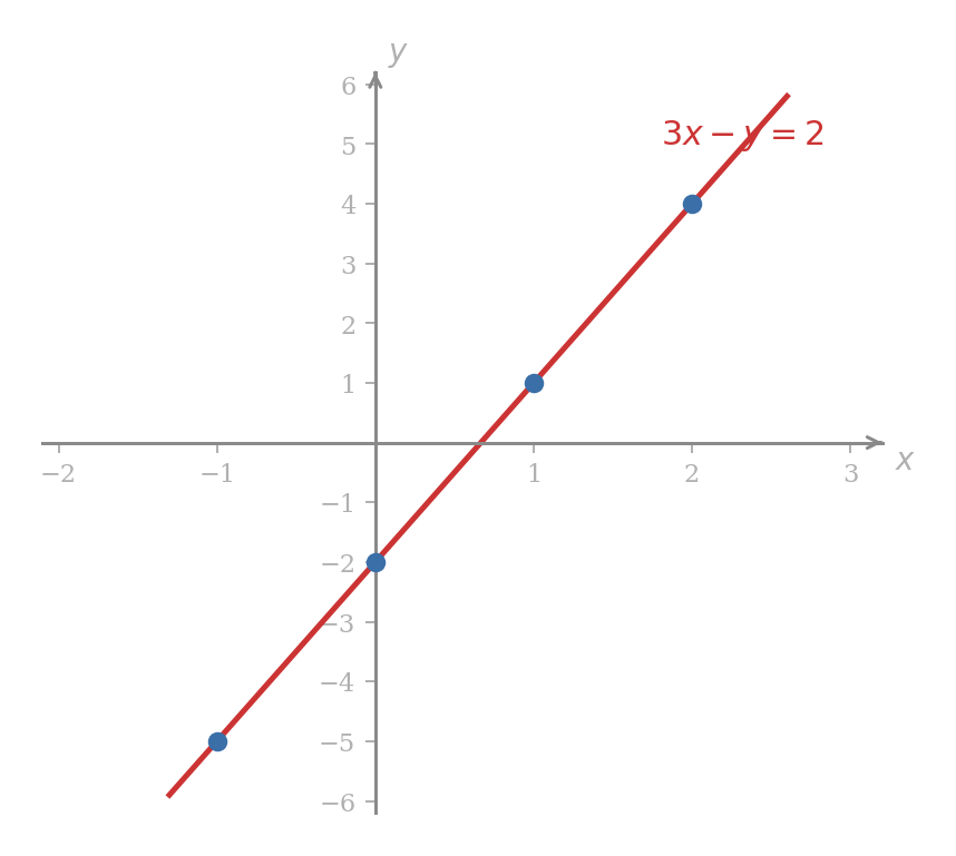
The vertical line x = a drawn as a straight vertical segment through (a, 0), with two sample points at different heights on the line both having the same x-coordinate a, illustrating that a single input corresponds to more than one output

Example 23

From a general equation to a sketch. To sketch the line $3x - y = 2$ , first solve for $y$ :

y = 3x - 2.

The equation is now in the form of the AM Linear Function definition, with slope $3$ and $y$ -intercept $-2$ . Tabulating at four inputs to verify the slope and give a cleaner sketch,

x	-1	0	1	2
y	-5	-2	1	4

each unit step in $x$ raises $y$ by exactly $3$ , consistent with the slope. The graph is the straight line through these points.

The straight line 3x - y = 2 drawn through the points (-1, -5), (0, -2), (1, 1), (2, 4), with each tabulated point marked

Problem 11

Put the equation $x = 2y - 1$ in the form $y = mx + b$ , identify its slope and its $y$ -intercept, and sketch the resulting line.

Intercepts

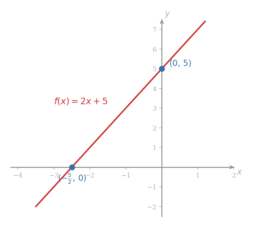
The AM Linear Function definition already names the point at which the line meets the vertical axis: if $f(x) = mx + b$ , then $f(0) = b$ , so the $y$ -intercept is $(0, b)$ . The corresponding point on the horizontal axis has not yet been named.

Definition 8 (

x

-intercept)

An $x$ -intercept of the graph of a function $f$ is a point at which the graph meets the horizontal axis. Every point of the horizontal axis has $y$ -coordinate zero, so an $x$ -intercept has the form $(x_0, 0)$ where $x_0$ is a real number in the domain of $f$ satisfying $f(x_0) = 0$ .

For a non-horizontal linear function $f(x) = mx + b$ with $m \neq 0$ , the equation $mx + b = 0$ has the single solution $x_0 = -b/m$ , so the graph has exactly one $x$ -intercept, namely $(-b/m, 0)$ . If $m = 0$ and $b \neq 0$ the graph is a horizontal line at height $b \neq 0$ and has no $x$ -intercept; if $m = 0$ and $b = 0$ the graph is the horizontal axis itself, and every one of its points is an $x$ -intercept.

Example 24

Both intercepts of $f(x) = 2x + 5$ . Reading off the definition, the $y$ -intercept is $(0, f(0)) = (0, 5)$ . For the $x$ -intercept we solve $2x + 5 = 0$ , which gives $x_0 = -\tfrac{5}{2}$ , so the $x$ -intercept is $(-\tfrac{5}{2}, 0)$ . The two intercepts alone pin down the line.

The line f(x) = 2x + 5 drawn with its y-intercept at (0, 5) and its x-intercept at (-5/2, 0) both highlighted and labelled

Example 25

Reconstructing a line from two intercepts. Suppose a line is known to pass through $(0, -4)$ and $(3, 0)$ . These are, respectively, its $y$ -intercept and an $x$ -intercept, so $b = -4$ and the slope is the rise $0 - (-4) = 4$ divided by the run $3 - 0 = 3$ , that is $m = \tfrac{4}{3}$ . The line is $f(x) = \tfrac{4}{3} x - 4$ .

Problem 12

Find both intercepts of the line $4x + 3y = 12$ and sketch it using only those two points.

Linear Models

Linear functions earn their prominence from the many real-world quantities that depend on one another by a constant rate plus a fixed offset. The derivative, which the lessons ahead will introduce, generalises the idea of a rate to curved graphs; the linear case is the template.

Example 26

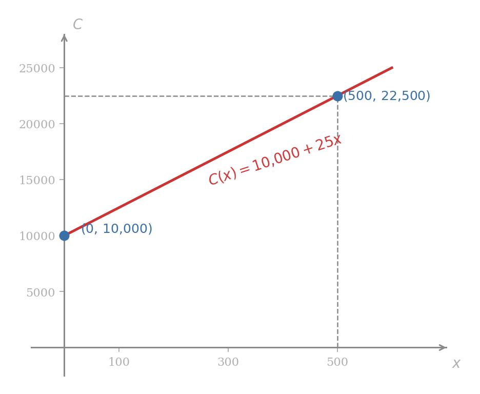
A monthly cost. A small publisher prints a bound booklet at a reproduction cost of $\pounds 25$ per copy and pays fixed overheads of $\pounds 10{,}000$ each month for premises, licences, and staff retainers that do not depend on the run size. Writing $x$ for the number of copies produced in a month and $C(x)$ for the total cost in pounds,

C(x) = 10{,}000 + 25 x.

The fixed overheads supply the $y$ -intercept $(0, 10{,}000)$ , while the $\pounds 25$ per-copy charge supplies the slope. At a run of $500$ copies,

C(500) = 10{,}000 + 25 \cdot 500 = 22{,}500 \text{ pounds}.

Since $x$ counts physical copies, the admissible inputs are the non-negative integers; the formula is nevertheless defined on the full ray $[0, \infty)$ , and we draw the graph there for readability.

The graph of the linear cost function C(x) = 10000 + 25x, rising from (0, 10000) through the marked sample point (500, 22500), with dashed lines dropped from that sample point to both axes

Problem 13

A courier has a fixed daily charge of $\pounds 12$ and a per-kilometre rate of $\pounds 0.40$ . Write the total daily charge $D(x)$ for a route of $x$ kilometres as a linear function, state its slope and $y$ -intercept, and compute $D(80)$ .

Piecewise Linear Functions

The piecewise construction introduced in the AM lesson, combined with the linear functions just revisited, gives a flexible class of graphs: straight on each piece of the domain and potentially bending or jumping at the boundaries. Such functions arise whenever one linear rule is replaced by another past a threshold, as in tariffs, tax brackets, and shipping charges.

Example 27

A piecewise linear function with a jump. Define

f(x) = \begin{cases} 3, & x < 2, \\ 2x + 1, & x \geq 2. \end{cases}

For $x$ strictly less than $2$ the top clause applies and the function is constantly $3$ , so the graph is the horizontal ray at height $3$ approaching but not reaching the point $(2, 3)$ ; the endpoint is drawn with an unfilled circle by the convention of the AM lesson. For $x \geq 2$ the bottom clause applies; at the boundary $f(2) = 2 \cdot 2 + 1 = 5$ , drawn as a filled circle, and the graph continues to the right as the linear ray of slope $2$ through $(2, 5)$ . Three sample values,

f(0) = 3, \qquad f(2) = 5, \qquad f(4) = 9,

confirm the switchover.

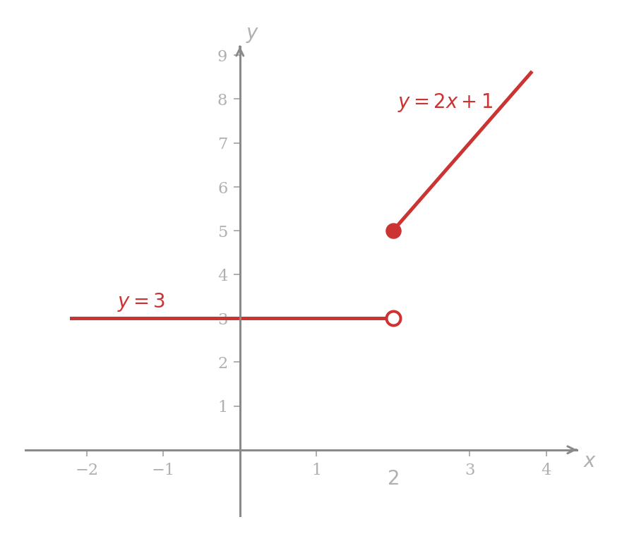
A piecewise graph: the horizontal line y = 3 for x less than 2 with an unfilled circle at (2, 3), and the line y = 2x + 1 for x greater than or equal to 2 with a filled circle at (2, 5); a visible vertical gap separates the two pieces at x = 2

Remark

The visible gap between the two pieces at $x = 2$ is a jump. The idea will return in the lessons ahead as the simplest way a function can fail to be continuous, and in turn to be differentiable. Piecewise linear functions are therefore our first and cleanest laboratory for the questions differentiation will ask.

Problem 14

Let

g(x) = \begin{cases} -x + 4, & x \leq 0, \\ x + 4, & x > 0. \end{cases}

Sketch the graph of $g$ , state its natural domain, and compute $g(-3)$ , $g(0)$ , and $g(5)$ . Does the graph have a jump at $x = 0$ ?

Problem 15

A phone plan charges $\pounds 15$ per month for up to $100$ minutes of calls, and $\pounds 0.10$ for each additional minute beyond the first hundred. Writing $M(t)$ for the monthly charge in pounds as a function of the total call minutes $t \geq 0$ , express $M$ as a piecewise function on $[0, \infty)$ and compute $M(60)$ and $M(250)$ .

Quadratic Functions

The parabola $y = x^2$ of the AM lesson is the simplest instance of a broader family. Quadratic functions arise as the first curved graphs for which the vertex, the intercepts, and the direction of opening are recoverable from the formula alone, and they will be the first curved graphs whose tangent lines the derivative will compute.

Definition 9 (Quadratic Function)

A quadratic function is a function of the form $f(x) = ax^2 + bx + c$ , where $a$ , $b$ , $c$ are real constants and $a \neq 0$ . Its natural domain is the whole number line. The graph of a quadratic function is called a parabola; it opens upward when $a > 0$ and downward when $a < 0$ .

Every parabola has a single point at which the graph reverses direction, the highest point when the parabola opens downward and the lowest when it opens upward. Completing the square locates that point exactly.

Theorem 1 (Vertex of a Parabola)

Let $f(x) = ax^2 + bx + c$ with $a \neq 0$ . Then $f$ attains its extreme value at

x_0 = -\frac{b}{2a}, \qquad f(x_0) = c - \frac{b^2}{4a}.

The point

\left( -\frac{b}{2a},\; c - \frac{b^2}{4a} \right)

is called the vertex of the parabola.

Proof

Completing the square on the leading two terms of $f$ ,

f(x) = a \left( x^2 + \frac{b}{a} x \right) + c = a \left( x + \frac{b}{2a} \right)^{2} - a \cdot \frac{b^2}{4a^2} + c = a \left( x + \frac{b}{2a} \right)^{2} + c - \frac{b^2}{4a}.

The squared factor is non-negative and vanishes precisely when $x = -b/(2a)$ . If $a > 0$ , the first summand is non-negative and so $f(x) \geq c - b^2/(4a)$ for every $x$ , with equality at $x = -b/(2a)$ ; the extreme value is therefore a minimum. If $a < 0$ , the first summand is non-positive and the same calculation yields a maximum at the same $x$ . In either case $f(-b/(2a)) = c - b^2/(4a)$ , which is the claim.

■

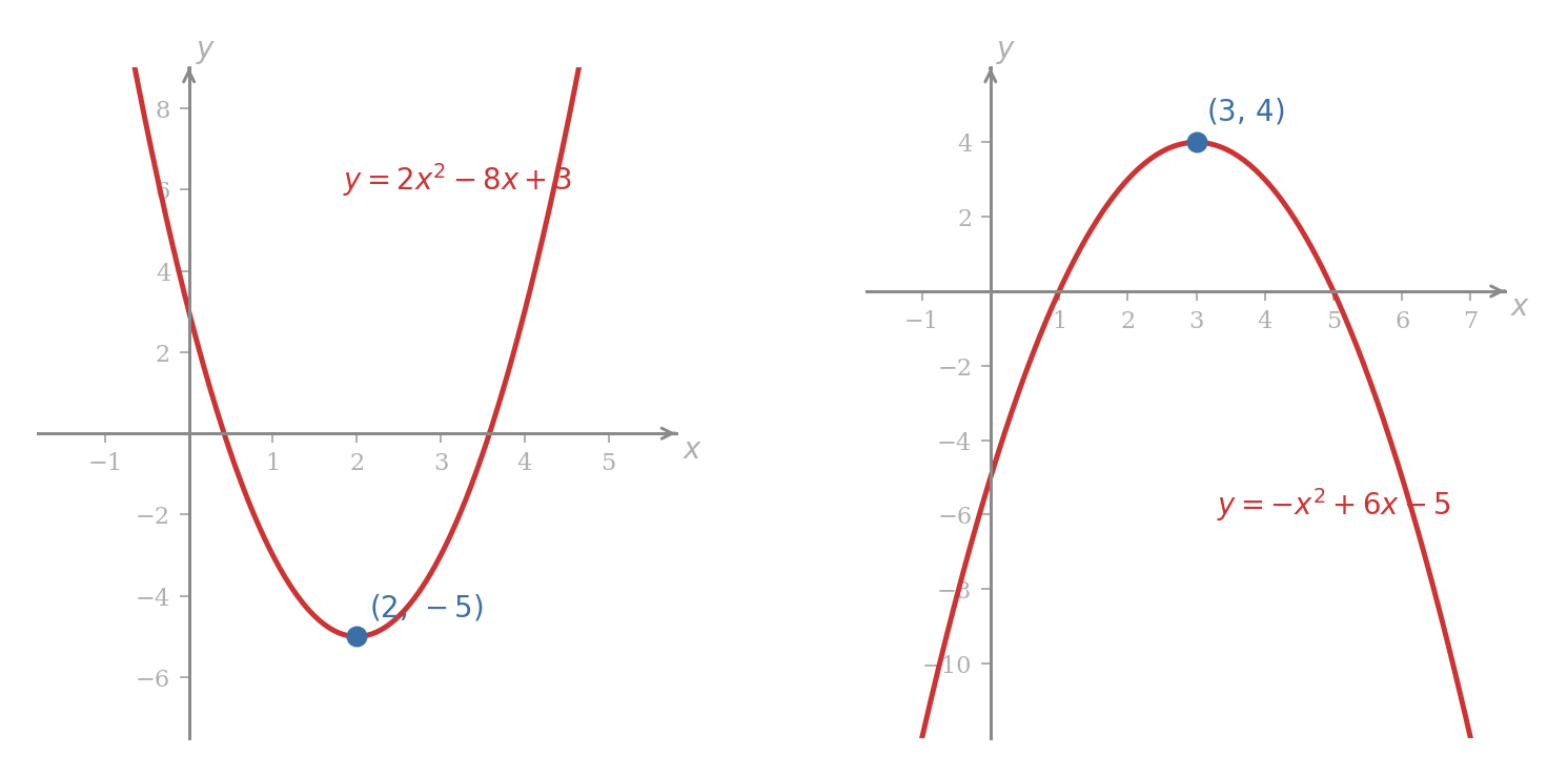
Two parabolas side by side: on the left y = 2x squared minus 8x plus 3 opening upward with its vertex at (2, -5) marked, on the right y = negative x squared plus 6x minus 5 opening downward with its vertex at (3, 4) marked

Example 28

Vertex of $f(x) = 2x^2 - 8x + 3$ . Here $a = 2$ , $b = -8$ , $c = 3$ , and the vertex formula gives

x_0 = -\frac{-8}{2 \cdot 2} = 2, \qquad f(2) = 2 \cdot 4 - 16 + 3 = -5.

So the vertex is $(2, -5)$ . Since $a = 2 > 0$ , the parabola opens upward and $-5$ is the minimum value of $f$ .

Example 29

A downward-opening parabola. For $f(x) = -x^2 + 6x - 5$ , we have $a = -1$ , $b = 6$ , $c = -5$ , so

x_0 = -\frac{6}{-2} = 3, \qquad f(3) = -9 + 18 - 5 = 4.

The vertex is $(3, 4)$ , and because $a < 0$ this is a maximum.

Problem 16

Find the vertex of $f(x) = 3x^2 + 12x + 7$ and state whether it is a maximum or a minimum. Compute the $y$ -intercept as well.

Remark

Techniques for sketching a parabola from more general data will follow at once from the first derivative. Until then, the vertex together with the $y$ -intercept $(0, c)$ is usually enough to fix the shape by eye, provided the two points are distinct; when the vertex happens to lie on the $y$ -axis the two points coincide and one further value of $f$ is needed.

Polynomial and Rational Functions

Linear and quadratic functions share a single template: a finite sum of non-negative integer powers of $x$ weighted by constants. Isolating the template gives the family within which most of the functions in this course will live.

Definition 10 (Polynomial Function)

A polynomial function is a function of the form

f(x) = a_n x^n + a_{n-1} x^{n-1} + \cdots + a_1 x + a_0,

where $n$ is a non-negative integer and $a_0, a_1, \ldots, a_n$ are real constants. Its natural domain is the whole number line, since every operation in the formula is addition or multiplication of real numbers.

The AM linear functions are the polynomial functions with $n \leq 1$ , and the quadratic functions of the previous section are the polynomial functions with $n = 2$ and $a_2 \neq 0$ .

Example 30

Each of

f(x) = 5x^3 - 3x^2 - 2x + 4, \qquad g(x) = x^4 - x + 1

is a polynomial function. Each is defined at every real number and is built from powers of $x$ by the permitted arithmetic.

Taking quotients of polynomial functions produces the first systematic exclusions from the natural domain.

Definition 11 (Rational Function)

A rational function is a function expressible as a quotient $p(x)/q(x)$ of polynomial functions $p$ and $q$ , where $q$ is not the zero polynomial. By the natural domain convention of the AM lesson, its admissible inputs are exactly those real $x$ at which $q(x) \neq 0$ .

Example 31

For

h(x) = \frac{x^2 + 1}{x}, \qquad k(x) = \frac{x + 3}{x^2 - 4},

the respective denominators vanish at $x = 0$ and at $x = \pm 2$ . The natural domain of $h$ is therefore every real $x \neq 0$ , and the natural domain of $k$ is every real $x$ with $x \neq 2$ and $x \neq -2$ .

Example 32

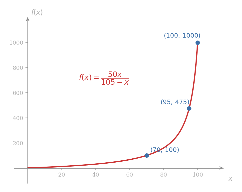
A cost-benefit model. Atmospheric scrubbers that remove a pollutant become disproportionately expensive as the residual fraction falls towards zero. A standard rational model for the cumulative cost is

f(x) = \frac{50 x}{105 - x}, \qquad 0 \leq x \leq 100,

where $x$ is the percentage of pollutant removed and $f(x)$ the cost in millions of dollars. The denominator vanishes only at $x = 105$ , outside the stated domain, so every admissible $x$ is genuinely assigned a real value. Direct substitution gives

f(70) = \frac{50 \cdot 70}{35} = 100, \qquad f(95) = \frac{50 \cdot 95}{10} = 475, \qquad f(100) = \frac{50 \cdot 100}{5} = 1000.

Thus removing $70\%$ of the pollutant costs 100 million dollars. The cost of removing the final $5\%$ , from $95\%$ to $100\%$ , is

f(100) - f(95) = 1000 - 475 = 525 \text{ million dollars},

over five times the cost of removing the first $70\%$ .

The graph of the cost-benefit function f(x) = 50x over 105 minus x on the domain from 0 to 100, curving gently upward near the origin and rising steeply as x approaches 100, with the sample points (70, 100), (95, 475), and (100, 1000) marked on the curve

Problem 17

With $f(x) = 50x/(105 - x)$ on $[0, 100]$ as in the example, compute the additional cost of raising the removal percentage from $70\%$ to $75\%$ , and compare the result with the cost of removing the final $5\%$ from $95\%$ to $100\%$ .

Power Functions

A further family sits between the polynomial and the rational: functions given by a single power of the variable.

Definition 12 (Power Function)

A power function is a function of the form $f(x) = x^r$ , where $r$ is a fixed real constant called the exponent.

When $r$ is a positive integer, $x^r$ denotes the product of $x$ with itself $r$ times and is defined for every real $x$ , so the power function is a polynomial function and its natural domain is the whole number line. When $r$ is a negative integer, $x^r$ means $1/x^{|r|}$ , and the natural domain excludes $x = 0$ . The meaning of $x^r$ for non-integer $r$ , together with the resulting natural domain, will be recovered in a later lesson.

The Absolute Value Function

One function of this lesson is neither polynomial nor rational nor a single power, but it fits the piecewise construction of the AM lesson exactly.

Definition 13 (Absolute Value)

The absolute value of a real number $x$ is the real number

|x| = \begin{cases} x, & x \geq 0, \\ -x, & x < 0, \end{cases}

and is non-negative for every $x$ .

Thus $|5| = 5$ , $|0| = 0$ , and $|-3| = -(-3) = 3$ . Regarding $|x|$ as a rule assigning each real $x$ a single real output gives a function in the sense of the AM Function definition.

Definition 14 (Absolute Value Function)

The absolute value function is the function $f(x) = |x|$ , with natural domain the whole number line. Its graph is the piecewise combination of the line $y = x$ on $[0, \infty)$ with the line $y = -x$ on $(-\infty, 0)$ , the two pieces meeting at the origin.

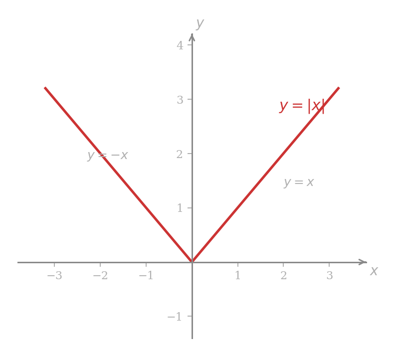
The graph of y = |x|, a V-shape meeting at the origin, with the left arm following the line y = -x and the right arm following the line y = x

The two pieces agree in value at $x = 0$ , so the graph does not jump in the sense introduced in the piecewise-linear section above; instead it has a sharp corner. This corner will reappear in a coming lesson as the first example of a function that is everywhere continuous but fails to be differentiable at a point.

Example 33

Evaluating at three inputs, $f(-7) = 7$ , $f(0) = 0$ , and $f(2.5) = 2.5$ . The non-negativity $|x| \geq 0$ for every $x$ follows directly from the two cases: when $x \geq 0$ the output is $x \geq 0$ ; when $x < 0$ the output is $-x > 0$ .

Problem 18

Sketch the graph of $f(x) = |x - 2|$ by applying a horizontal shift from the AM lesson to the absolute value function, and state its $x$ - and $y$ -intercepts.

Combining Functions

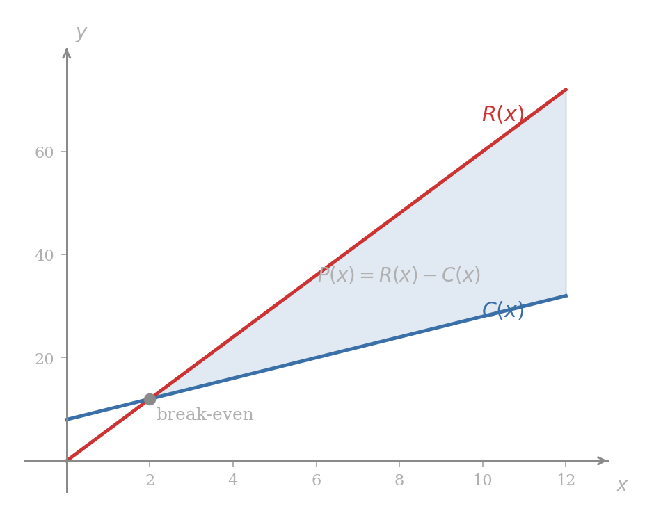
Many functions of practical interest are assembled from simpler ones by arithmetic. The prototype is a firm’s profit: if $R(x)$ is the revenue from selling $x$ units of a commodity and $C(x)$ is the cost of producing those $x$ units, the profit on the sale is

P(x) = R(x) - C(x).

Writing $P$ in this form turns questions about profit into questions about the comparison of $R$ and $C$ . The firm runs at a profit on exactly those inputs $x$ at which $R(x) > C(x)$ , and the graph of $P$ lies above the horizontal axis precisely where the graph of $R$ lies above the graph of $C$ .

Two straight lines on the same axes: revenue R(x) rising steeply from the origin and cost C(x) rising less steeply from a positive y-intercept; the two lines cross at a break-even point, with the region beyond it where R exceeds C shaded to represent the profit

The construction generalises to the other three arithmetic operations.

Definition 15 (Sum, Difference, Product, Quotient of Functions)

Let $f$ and $g$ be functions. Their sum, difference, product, and quotient are the functions defined pointwise by

(f + g)(x) = f(x) + g(x), \qquad (f - g)(x) = f(x) - g(x),

(f g)(x) = f(x) g(x), \qquad \left( \frac{f}{g} \right)(x) = \frac{f(x)}{g(x)}.

The natural domain of each of $f + g$ , $f - g$ , and $fg$ is the intersection of the natural domains of $f$ and $g$ . The natural domain of $f/g$ is that same intersection, with the additional exclusion of every $x$ at which $g(x) = 0$ .

Addition, subtraction, and multiplication of functions are nothing but the corresponding operations on their values, admissible wherever both values are admissible. The quotient brings back the exclusion already familiar from the rational function section: the divisor must not vanish.

Fraction arithmetic

Before working examples, the five rules of fraction arithmetic needed in the sequel are worth stating in one place. Every letter appearing in a denominator is understood to be non-zero throughout.

Theorem 2 (Rules for Fractions)

For real numbers $a, b, c, d$ with $b, c, d$ non-zero as required,

\text{(i)} \quad a \cdot \frac{b}{c} = \frac{ab}{c}, \qquad \text{(ii)} \quad \frac{a}{b} \cdot \frac{c}{d} = \frac{ac}{bd},

\text{(iii)} \quad \frac{ac}{bc} = \frac{a}{b}, \qquad \text{(iv)} \quad \frac{a/b}{c/d} = \frac{a}{b} \cdot \frac{d}{c} = \frac{ad}{bc},

\text{(v)} \quad \frac{a}{b} + \frac{c}{d} = \frac{ad + bc}{bd}.

Rule (iii) is most often applied in reverse: cancellation of a factor common to numerator and denominator. Rule (v) is the addition rule via a common denominator and is the single rule required for combining rational functions with different denominators.

A worked example: linear combinations

Example 34

Let $f(x) = 2x + 4$ and $g(x) = 2x - 6$ . We compute the sum, difference, product, and quotient in their simplest forms.

For the sum and difference, corresponding terms are added or subtracted:

(f + g)(x) = (2x + 4) + (2x - 6) = 4x - 2,

(f - g)(x) = (2x + 4) - (2x - 6) = 10.

The difference is a constant: the graphs of $f$ and $g$ are parallel lines, each of slope $2$ , separated by $10$ units vertically.

For the product, expand by distributing each term of the first factor across each term of the second:

(f g)(x) = (2x + 4)(2x - 6) = 4x^2 - 12x + 8x - 24 = 4x^2 - 4x - 24.

The four summands are, in order, the product of the First terms, the Outer terms, the Inner terms, and the Last terms; this order is commonly remembered by the acronym FOIL.

For the quotient, substitute the formulas and then factorise numerator and denominator before cancelling:

\frac{f(x)}{g(x)} = \frac{2x + 4}{2x - 6} = \frac{2(x + 2)}{2(x - 3)} = \frac{x + 2}{x - 3},

using rule (iii) to cancel the common factor of $2$ . Cancellation is legitimate here only because $2$ is a genuine factor of every term in both numerator and denominator; the tempting move of cancelling the $2x$ that appears in both is invalid, because $2x$ is not a factor of either expression but merely one term in a sum. The natural domain of the quotient is every real $x$ with $g(x) \neq 0$ , that is, every $x \neq 3$ .

Problem 19

Let $f(x) = x^2 + 1$ , $g(x) = 9x$ , and $h(x) = 5 - 2x^2$ . Compute each of the following, simplified to standard form, and state the natural domain in each case.

$(f + g)(x)$
$(f - h)(x)$
$(f g)(x)$
$\dfrac{g(x)}{f(x)}$

Adding rational functions

Rule (v) says that two fractions are added by passing to a common denominator. For rational functions the procedure is identical, with $x$ in place of the real letters.

Example 35

Let

g(x) = \frac{2}{x}, \qquad h(x) = \frac{3}{x - 1}.

The natural domain of $g$ excludes $x = 0$ and the natural domain of $h$ excludes $x = 1$ , so the previous definition gives the natural domain of $g + h$ as the real line with both of these points removed. On that common domain, multiply each fraction by whatever unit fraction is needed to reach the common denominator $x(x - 1)$ :

g(x) + h(x) = \frac{2}{x} \cdot \frac{x - 1}{x - 1} + \frac{3}{x - 1} \cdot \frac{x}{x} = \frac{2(x - 1)}{x(x - 1)} + \frac{3x}{x(x - 1)}.

The two fractions now share the denominator $x(x - 1)$ and combine directly:

g(x) + h(x) = \frac{2(x - 1) + 3x}{x(x - 1)} = \frac{5x - 2}{x(x - 1)}.

The result is a rational function in the sense of the previous section, defined at every real $x$ distinct from $0$ and from $1$ .

Problem 20

Let $f(x) = \dfrac{x}{x - 8}$ and $g(x) = \dfrac{-x}{x - 4}$ . Express $f(x) + g(x)$ as a single rational function in simplest form, state its natural domain, and find the real $x$ at which the numerator vanishes.

Problem 21

A firm selling $x$ units of a commodity earns revenue $R(x) = 40x$ pounds and incurs cost $C(x) = 5x + 200$ pounds, valid for $x \geq 0$ . Write the profit $P(x) = R(x) - C(x)$ as a linear function, determine the break-even quantity at which $P(x) = 0$ , and state the collection of $x$ for which the firm makes a strictly positive profit.

Multiplying and dividing rational functions

The remaining two operations on rational functions follow rules (ii) and (iv) directly.

Example 36

Multiplying. For

f(t) = \frac{t}{t - 1}, \qquad g(t) = \frac{t + 2}{t + 1},

rule (ii) gives the product as numerator times numerator over denominator times denominator:

f(t) g(t) = \frac{t(t + 2)}{(t - 1)(t + 1)}.

Expanding both numerator and denominator produces an equivalent expression:

f(t) g(t) = \frac{t^2 + 2t}{t^2 - 1}.

The two forms are the same function; whichever one is used depends on the purpose. The factored form makes the excluded inputs visible at a glance, namely $t \neq 1$ and $t \neq -1$ , while the expanded form is occasionally more convenient for comparing coefficients.

Example 37

Dividing. For

f(x) = \frac{x}{x - 3}, \qquad g(x) = \frac{x + 1}{x - 5},

the natural domain of $f$ excludes $x = 3$ and the natural domain of $g$ excludes $x = 5$ . For the quotient $f/g$ we must additionally exclude every $x$ at which $g(x) = 0$ , which occurs exactly when $x + 1 = 0$ , that is, $x = -1$ . The natural domain of $f/g$ therefore consists of every real $x$ with $x \neq -1$ , $3$ , $5$ .

On that domain, rule (iv) turns division into multiplication by the reciprocal:

\frac{f(x)}{g(x)} = \frac{x}{x - 3} \cdot \frac{x - 5}{x + 1} = \frac{x(x - 5)}{(x - 3)(x + 1)}.

Expanding gives the equivalent expression

\frac{f(x)}{g(x)} = \frac{x^2 - 5x}{x^2 - 2x - 3}.

Composition of Functions

The AM lesson already noted that any expression whose value is a real number may serve as the input of a function, and that most of the course’s functions are assembled by evaluating one inside another. Naming this construction cleanly is overdue.

Definition 16 (Composition)

Let $f$ and $g$ be functions. The composition of $f$ with $g$ , written $f \circ g$ or $f(g(x))$ , is the function defined by

(f \circ g)(x) = f(g(x)).

Its natural domain consists of every real $x$ in the natural domain of $g$ for which the value $g(x)$ lies in the natural domain of $f$ .

The value $g(x)$ of the inner function must be an admissible input of the outer function, so the natural domain of $f \circ g$ is in general smaller than that of $g$ . Order matters: $f \circ g$ and $g \circ f$ are different functions in most cases, and the example below demonstrates the point.

Example 38

Let $f(x) = x^2 + 3x + 1$ and $g(x) = x - 5$ . Substituting $g(x) = x - 5$ for every occurrence of $x$ in the formula for $f$ ,

\begin{aligned} f(g(x)) &= (x - 5)^2 + 3(x - 5) + 1 \\ &= (x^2 - 10x + 25) + (3x - 15) + 1 \\ &= x^2 - 7x + 11. \end{aligned}

Substituting $f(x) = x^2 + 3x + 1$ for every occurrence of $x$ in the formula for $g$ ,

g(f(x)) = (x^2 + 3x + 1) - 5 = x^2 + 3x - 4.

The two outputs are different polynomial functions, confirming that composition is not commutative in general.

Problem 22

Let $f(x) = \sqrt{x}$ and $g(x) = 1 - x^2$ . Compute $f(g(x))$ and $g(f(x))$ , and state the natural domain of each.

The difference quotient

A particularly important composition takes the inner function to be a horizontal shift of the variable, $g(x) = x + h$ for a fixed real $h$ . Then $(f \circ g)(x) = f(x + h)$ , the quantity that already drove the horizontal shift construction of the AM lesson. Combining this composition with the subtraction and division of the previous section produces the single expression in which the derivative, the object of the lessons ahead, will be born.

Definition 17 (Difference Quotient)

Let $f$ be a function and let $h$ be a non-zero real number. The difference quotient of $f$ at $x$ with increment $h$ is

\frac{f(x + h) - f(x)}{h}.

It is defined at every $x$ for which both $x$ and $x + h$ lie in the natural domain of $f$ .

The numerator is the change in the value of $f$ as the input moves from $x$ to $x + h$ . Dividing by $h$ converts that change into a rate per unit increment. The derivative will be recovered by driving $h$ to zero.

Example 39

Difference quotient of $f(x) = x^3$ . Using the cube expansion, obtained by two applications of FOIL,

f(x + h) = (x + h)^3 = x^3 + 3 x^2 h + 3 x h^2 + h^3.

Subtracting $f(x) = x^3$ ,

f(x + h) - f(x) = 3 x^2 h + 3 x h^2 + h^3.

Every summand carries a factor of $h$ , so factoring it out and applying rule (iii) under the assumption $h \neq 0$ ,

\frac{f(x + h) - f(x)}{h} = \frac{h(3 x^2 + 3 x h + h^2)}{h} = 3 x^2 + 3 x h + h^2.

Cancellation is legitimate because $h \neq 0$ ; at $h = 0$ the original quotient is undefined, but the simplified expression remains meaningful and equals $3 x^2$ .

Remark

The value $3 x^2$ left over after the cancellation will turn out, in a coming lesson, to be the derivative of $x^3$ . The algebra of this section therefore already delivers the derivative of the cube, pending only the limit argument that makes the passage from $h \neq 0$ to $h = 0$ rigorous. The pattern repeats for every polynomial: the difference quotient factors, $h$ cancels, and what remains is the derivative. The whole of differentiation lives in that cancellation.

Problem 23

Let $f(x) = x^2$ . Form the difference quotient $\dfrac{f(x + h) - f(x)}{h}$ , simplify it using $h \neq 0$ , and state the value of the simplified expression at $h = 0$ .

Problem 24

Let $f(x) = \dfrac{1}{x}$ with $x \neq 0$ , and suppose also that $x + h \neq 0$ . Express the difference quotient

\frac{f(x + h) - f(x)}{h}

as a single rational function of $x$ and $h$ in simplest form, and state the value of the simplified expression at $h = 0$ .