16/03/2026

#Math#Differentiation

Lesson assets

No linked assets.

Quadratics, Factoring, and Rational Exponents

Zeros of a Function

The PM lesson named the point at which the graph of $f$ meets the horizontal axis: the $x$ -intercept. In practice we also need a name for the input that produces it, independently of the graph.

Definition 1 (Zero of a Function)

A zero (or root) of a function $f$ is a real number $x_0$ in the domain of $f$ with $f(x_0) = 0$ . The $x$ -intercepts of the graph of $f$ are exactly the points $(x_0, 0)$ for which $x_0$ is a zero of $f$ .

Locating the zeros of $f$ therefore locates the $x$ -intercepts of its graph, but the use goes further. Two graphs $y = f(x)$ and $y = g(x)$ meet at precisely those $x$ with $f(x) = g(x)$ , and writing $h = f - g$ in the sum-difference sense of the PM lesson converts this to the single condition $h(x) = 0$ . The break-even inputs of a profit function $P = R - C$ are exactly the zeros of $P$ . Every question of the form where does one quantity cross another reduces to finding zeros of a suitable combination of functions.

The PM lesson has already supplied the zeros of every linear function: if $f(x) = mx + b$ with $m \neq 0$ , then the unique zero is $x_0 = -b/m$ . The next non-trivial case is the quadratic, and for it the technique of completing the square produces a closed formula.

The Quadratic Formula

Theorem 1 (Quadratic Formula)

Let $a, b, c$ be real with $a \neq 0$ . The real zeros of the quadratic function $f(x) = ax^2 + bx + c$ are precisely the real solutions of the equation $ax^2 + bx + c = 0$ , and they are given by

x = \frac{-b \pm \sqrt{b^2 - 4ac}}{2a}.

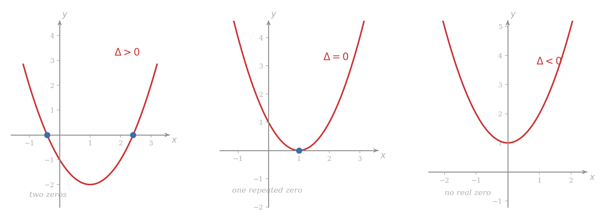
The quantity $\Delta = b^2 - 4ac$ is called the discriminant. The equation has two distinct real solutions when $\Delta > 0$ , a single repeated real solution when $\Delta = 0$ , and no real solution when $\Delta < 0$ .

Proof

Start from $ax^2 + bx + c = 0$ , move the constant across, and multiply both sides by $4a$ , which is non-zero because $a \neq 0$ ,

4a^2 x^2 + 4abx = -4ac.

Adding $b^2$ to both sides completes the square on the left,

4a^2 x^2 + 4abx + b^2 = b^2 - 4ac,

since $(2ax + b)^2 = 4a^2 x^2 + 4abx + b^2$ by direct expansion. Hence

(2ax + b)^2 = b^2 - 4ac.

When $b^2 - 4ac < 0$ the left side, a square of a real number, cannot equal a negative number and so the equation has no real solution. When $b^2 - 4ac \geq 0$ the square root on the right is real, and the equation is equivalent to

2ax + b = \pm \sqrt{b^2 - 4ac}.

Solving for $x$ gives the stated formula. The two signs coincide exactly when $b^2 - 4ac = 0$ , producing a single repeated solution in that case and two distinct solutions otherwise.

■

The discriminant $\Delta = b^2 - 4ac$ governs the geometry. A parabola with two zeros crosses the horizontal axis at two distinct points; a parabola with one zero meets it tangentially at its vertex; a parabola with no real zero sits entirely above or entirely below the axis, according to the sign of $a$ .

Three parabolas shown side by side illustrating the three discriminant cases: on the left a parabola crossing the x-axis at two distinct points, in the middle a parabola touching the x-axis at a single point with its vertex on the axis, and on the right a parabola lying entirely above the x-axis

Example 1 (Two distinct zeros)

Solving $2x^2 - 5x + 1 = 0$ . Here $a = 2$ , $b = -5$ , $c = 1$ , so

\Delta = (-5)^2 - 4 \cdot 2 \cdot 1 = 25 - 8 = 17 > 0,

and the formula gives

x = \frac{5 \pm \sqrt{17}}{4}.

The two zeros are $\tfrac{5 + \sqrt{17}}{4} \approx 2.28$ and $\tfrac{5 - \sqrt{17}}{4} \approx 0.22$ .

Example 2 (A single repeated zero)

Solving $9x^2 - 12x + 4 = 0$ . Here $a = 9$ , $b = -12$ , $c = 4$ , so

\Delta = 144 - 144 = 0,

and the formula collapses to a single solution,

x = \frac{12}{18} = \frac{2}{3}.

The parabola $y = 9x^2 - 12x + 4$ therefore has its vertex on the horizontal axis at $\left(\tfrac{2}{3}, 0\right)$ , a special case of the vertex formula from the PM lesson.

Example 3 (No real zero)

Solving $x^2 + 2x + 5 = 0$ . Here $a = 1$ , $b = 2$ , $c = 5$ , so

\Delta = 4 - 20 = -16 < 0,

and the equation has no real solution. The completed-square form

x^2 + 2x + 5 = (x + 1)^2 + 4 \geq 4

confirms that the graph sits at height at least $4$ above the horizontal axis, the minimum $4$ being attained at $x = -1$ .

Problem 1

For each of the quadratic functions below, compute the discriminant, classify the number of real zeros, and find them when they exist.

$f(x) = x^2 - 6x + 4$ .
$f(x) = 4x^2 + 4x + 1$ .
$f(x) = 3x^2 + x + 1$ .

Intersection of Graphs

Asking where two curves meet asks for the common solutions of a pair of equations in $x$ and $y$ . When both curves are graphs of functions of $x$ , the two equations can be equated to eliminate $y$ , reducing the problem to a single equation in $x$ alone; if the resulting equation is quadratic, the formula above resolves it completely.

Example 4 (A parabola meeting a line)

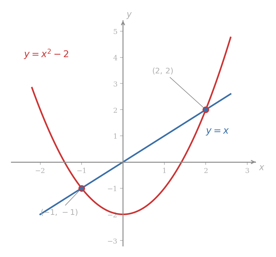
Find where the graphs of $y = x^2 - 2$ and $y = x$ meet. A point $(x, y)$ lies on both graphs exactly when $y = x^2 - 2$ and $y = x$ hold simultaneously. Equating the two expressions for $y$ ,

x^2 - 2 = x, \qquad \text{equivalently} \qquad x^2 - x - 2 = 0.

Here $a = 1$ , $b = -1$ , $c = -2$ , and $\Delta = 1 + 8 = 9$ , so

x = \frac{1 \pm 3}{2},

so $x = 2$ or $x = -1$ . Substituting each into the simpler equation $y = x$ gives the corresponding heights, and the two curves meet at $(2, 2)$ and $(-1, -1)$ .

The parabola y equals x squared minus 2 and the line y equals x drawn on the same axes, crossing at the two points (-1, -1) and (2, 2), with both intersection points marked and labelled

Problem 2

Find every intersection point of the graphs of $y = 2x^2$ and $y = 3x + 2$ , and verify your answer by substitution into each equation.

Factoring

The quadratic formula reduces every quadratic equation to arithmetic, but where factoring is available it is both faster and more informative, because it displays the zeros directly in the form of the expression. Its force comes from a single algebraic observation.

Remark (The product-zero principle)

A product of real numbers is zero if and only if at least one of its factors is zero. Applied to a polynomial written as a product of linear factors

f(x) = a\,(x - r_1)(x - r_2) \cdots (x - r_n), \qquad a \neq 0,

the principle says the zeros of $f$ are exactly the numbers $r_1, r_2, \ldots, r_n$ . The leading coefficient $a$ is excluded from being zero because setting $a = 0$ collapses $f$ to the zero function, every real number of which is a zero. Factoring a polynomial therefore reads off its zeros by inspection.

Factoring a quadratic by inspection

For a quadratic $x^2 + px + q$ with leading coefficient $1$ we look for integers $c, d$ with

(x + c)(x + d) = x^2 + (c + d)\,x + cd = x^2 + px + q.

Thus $c$ and $d$ must multiply to $q$ and sum to $p$ . The search terminates rapidly because $q$ has only finitely many integer factorisations.

Example 5 (Four quadratics with leading coefficient one)

$x^2 + 9x + 20$ . We need $cd = 20$ and $c + d = 9$ . Taking $c = 4$ , $d = 5$ works, so $x^2 + 9x + 20 = (x + 4)(x + 5)$ , and the zeros are $-4, -5$ .
$x^2 - 11x + 24$ . Both numbers must be negative, since their product is positive and their sum negative. Taking $c = -3$ , $d = -8$ gives $x^2 - 11x + 24 = (x - 3)(x - 8)$ .
$x^2 + 2x - 15$ . The two numbers have opposite signs, summing to $+2$ and multiplying to $-15$ . Taking $c = 5$ , $d = -3$ gives $x^2 + 2x - 15 = (x + 5)(x - 3)$ .
$x^2 - 2x - 15$ . The same pair with signs reversed gives $x^2 - 2x - 15 = (x - 5)(x + 3)$ .

When the leading coefficient is not $1$ , the quadratic $ax^2 + bx + c$ is most efficiently factored either by first pulling out any common factor from the three coefficients, or, when that fails and the discriminant $\Delta = b^2 - 4ac$ is non-negative, by applying the quadratic formula to read off its real zeros $r_1, r_2$ and writing

ax^2 + bx + c = a\,(x - r_1)(x - r_2).

When $\Delta < 0$ the quadratic has no real zeros and admits no factorisation into real linear factors.

Example 6 (Pulling out a common factor)

Factor $3x^2 - 21x + 30$ . Extracting $3$ from every coefficient,

3x^2 - 21x + 30 = 3\,(x^2 - 7x + 10) = 3\,(x - 5)(x - 2),

with the inner quadratic factored by inspection, since $(-5)(-2) = 10$ and $(-5) + (-2) = -7$ . The zeros are $5$ and $2$ .

Standard identities

A handful of algebraic identities recur frequently enough to deserve names. Each is verified by multiplying out the right-hand side.

Note (Standard factoring identities)

A^2 - B^2 = (A - B)(A + B) \qquad \text{(difference of squares)}

A^2 + 2AB + B^2 = (A + B)^2, \qquad A^2 - 2AB + B^2 = (A - B)^2 \qquad \text{(perfect squares)}

A^3 - B^3 = (A - B)(A^2 + AB + B^2) \qquad \text{(difference of cubes)}

A^3 + B^3 = (A + B)(A^2 - AB + B^2) \qquad \text{(sum of cubes)}

Example 7 (Using the standard identities)

$x^2 - 49 = x^2 - 7^2 = (x - 7)(x + 7)$ , by difference of squares.
$x^2 - 14x + 49 = x^2 - 2 \cdot 7 \cdot x + 7^2 = (x - 7)^2$ , by the second perfect-square identity.
$x^3 - 27 = x^3 - 3^3 = (x - 3)(x^2 + 3x + 9)$ , by difference of cubes.
$8x^3 + 1 = (2x)^3 + 1^3 = (2x + 1)(4x^2 - 2x + 1)$ , by sum of cubes.

Higher-degree polynomials

Beyond degree two the quadratic formula no longer applies directly, but extracting a common factor of $x$ (or of a higher power of $x$ ) often reduces the problem to a quadratic once pulled out.

Example 8 (A cubic with three rational zeros)

Factor $x^3 + 4x^2 - 12x$ . Every term carries a factor of $x$ , so

x^3 + 4x^2 - 12x = x\,(x^2 + 4x - 12) = x\,(x + 6)(x - 2),

the inner quadratic being factored by inspection since $6 \cdot (-2) = -12$ and $6 + (-2) = 4$ . The zeros are $0, -6, 2$ .

Example 9 (A cubic with an irrational zero)

Factor $x^3 - 7x$ . Pulling out $x$ and applying the difference-of-squares identity with $B = \sqrt{7}$ ,

x^3 - 7x = x\,(x^2 - 7) = x\,(x - \sqrt{7})(x + \sqrt{7}).

The zeros are $0, \sqrt{7}, -\sqrt{7}$ .

Problem 3

Factor each of the following over the real numbers, and list the zeros.

$x^2 - 36$ .
$x^2 - 8x + 16$ .
$2x^2 - 9x - 5$ .
$x^3 + 64$ .
$x^4 - 9x^2$ .

Rational Equations

A rational equation is an equation between two rational expressions in $x$ . By the rational-function convention of the PM lesson, each side is defined on the intersection of the natural domains of its constituents, so a candidate solution must lie in that intersection; any value at which an original denominator vanishes is forbidden in advance. The standard procedure is to clear denominators by multiplying through by a common denominator, solve the resulting polynomial equation, and then discard any candidate at which an original denominator vanishes.

Example 10 (A rational equation reducing to a quadratic)

Solve

\frac{1}{x} + \frac{1}{x + 2} = \frac{3}{4}.

The denominators $x$ and $x + 2$ vanish at $x = 0$ and $x = -2$ respectively, so both values are forbidden. A common denominator for the three fractions is $4x(x + 2)$ , and multiplying through by it,

4(x + 2) + 4x = 3x(x + 2).

Expanding both sides gives $8x + 8 = 3x^2 + 6x$ , which rearranges to

3x^2 - 2x - 8 = 0.

Here $a = 3$ , $b = -2$ , $c = -8$ , and $\Delta = 4 + 96 = 100$ , so

x = \frac{2 \pm 10}{6},

so $x = 2$ or $x = -\tfrac{4}{3}$ . Neither value is forbidden, so both are solutions, a fact a direct substitution into the original equation confirms.

Problem 4

Solve each equation, discarding any value at which an original denominator vanishes.

$\dfrac{2}{x - 1} = \dfrac{3}{x + 2}$ .
$\dfrac{1}{x} + \dfrac{1}{x + 1} = \dfrac{5}{6}$ .
$\dfrac{x^2 - 4x + 4}{x - 2} = 3$ .

Exponents and Power Functions

The PM lesson named the power function $f(x) = x^r$ and assigned a meaning to $x^r$ when $r$ is a positive or negative integer, leaving non-integer $r$ for later recovery. Rational exponents can be recovered now with very little extra effort, and once they are in place the familiar algebraic manipulations of $x^r$ become available for the rest of the course.

Rational exponents

Let $b$ be a real number. The meaning of $b^r$ when $r$ is a positive integer, or a negative integer with $b \neq 0$ , was fixed by the PM lesson. We extend the definition in stages.

Definition 2 (Zero Exponent)

For any non-zero real number $b$ , we set $b^0 = 1$ .

The value $0^0$ is left undefined throughout the course. The stipulation $b^0 = 1$ is chosen so that the rule $b^{r} b^{s} = b^{r + s}$ extends without exception to the case $s = 0$ : setting $s = 0$ on the right forces $b^r \cdot b^0 = b^r$ , and the only value of $b^0$ compatible with this equation for every $r$ is $1$ .

Definition 3 (Reciprocal Roots)

Let $n$ be a positive integer. When $b \geq 0$ , the symbol $b^{1/n}$ denotes the unique real number $y \geq 0$ satisfying $y^n = b$ . When $n$ is odd, this extends to every real $b$ : if $b < 0$ then $b^{1/n}$ denotes the unique real number $y$ satisfying $y^n = b$ , which is itself negative. When $n$ is even and $b < 0$ , no real $y$ satisfies $y^n = b$ , and $b^{1/n}$ is left undefined.

For $n = 2$ this recovers the square root already familiar from the AM lesson: $b^{1/2} = \sqrt{b}$ for $b \geq 0$ . Numerically, $4^{1/2} = 2$ , $27^{1/3} = 3$ , $(-8)^{1/3} = -2$ , while $(-4)^{1/2}$ is undefined.

Definition 4 (Rational Exponent)

Let $m$ and $n$ be positive integers with no common factor, and let $b$ be a real number for which $b^{1/n}$ is defined. Then

b^{m/n} = (b^{1/n})^m.

When $b^{m/n}$ is defined and non-zero, the negative rational exponent is defined by reciprocation,

b^{-m/n} = \frac{1}{b^{m/n}}.

The requirement that $m/n$ be in lowest terms matters when $b$ is negative. The same rational number can be written in many ways, and the definition of $b^{m/n}$ would disagree with itself if applied blindly. Take $(-8)^{2/6}$ : written with denominator $6$ , the formula asks for $((-8)^{1/6})^2$ , and $(-8)^{1/6}$ is undefined. Reducing $2/6$ to its lowest terms $1/3$ first, the formula returns the well-defined value $(-8)^{1/3} = -2$ . Enforcing lowest terms in the definition keeps the output single-valued.

Example 11 (Three numerical evaluations)

Working directly from the definition,

8^{5/3} = (8^{1/3})^5 = 2^5 = 32, \qquad 8^{-5/3} = \frac{1}{8^{5/3}} = \frac{1}{32},

while

(-8)^{5/3} = \bigl((-8)^{1/3}\bigr)^{5} = (-2)^5 = -32,

the evaluation being legitimate because the denominator $n = 3$ is odd, so $(-8)^{1/3}$ is defined.

Laws of Exponents

The integer laws familiar from arithmetic extend to every rational exponent for which both sides of each identity are defined.

Theorem 2 (Laws of Exponents)

Let $r$ and $s$ be rational numbers, and let $a$ , $b$ be positive real numbers. Then

\text{(i)}\quad b^{r} b^{s} = b^{r + s}, \qquad \text{(ii)}\quad b^{-r} = \frac{1}{b^{r}}, \qquad \text{(iii)}\quad \frac{b^{r}}{b^{s}} = b^{r - s},

\text{(iv)}\quad (b^{r})^{s} = b^{rs}, \qquad \text{(v)}\quad (ab)^{r} = a^{r} b^{r}, \qquad \text{(vi)}\quad \left(\frac{a}{b}\right)^{r} = \frac{a^{r}}{b^{r}}.

Rule (ii) is the definition of the negative exponent rewritten; rule (iii) follows from (i) and (ii) on replacing $s$ by $-s$ . The remaining laws reduce to the definitions once every expression is unfolded, and we take them for granted.

The positivity of $b$ (and of $a$ ) is essential: rule (iv), for instance, fails for negative bases even when both sides are defined. With $b = -8$ , $r = \tfrac{2}{3}$ , and $s = \tfrac{3}{2}$ ,

(b^{r})^{s} = \bigl((-8)^{2/3}\bigr)^{3/2} = 4^{3/2} = 8, \qquad \text{but} \qquad b^{rs} = (-8)^{1} = -8.

The two expressions disagree because $(-8)^{2/3}$ squares the cube root of $-8$ , destroying the minus sign, whereas $(-8)^{1}$ keeps it. The lowest-terms convention treats the exponents $\tfrac{2}{3} \cdot \tfrac{3}{2}$ and $1$ as different computational recipes, and the two recipes need not agree when $b < 0$ . For negative bases the laws are reliable only on a case-by-case basis; in the expressions that will arise in this course the base is almost always positive, and the blanket hypothesis above applies.

In the symbolic examples below, every simplification is read on the natural domain of the original expression. Thus a fractional power such as $x^{1/2}$ or $x^{3/2}$ implicitly requires $x \geq 0$ or $x > 0$ as appropriate, and a negative power such as $x^{-1}$ or $x^{-3}$ requires $x \neq 0$ .

Example 12 (Combining laws)

Part (a). Using law (v) followed by a direct evaluation,

2^{1/2} \cdot 50^{1/2} = (2 \cdot 50)^{1/2} = 100^{1/2} = 10.

Part (b). Using law (i) inside the bracket and law (iv) outside,

(2^{1/2} \cdot 2^{1/3})^6 = (2^{(1/2) + (1/3)})^6 = (2^{5/6})^6 = 2^{(5/6) \cdot 6} = 2^5 = 32.

Part (c). Writing $\sqrt{5} = 5^{1/2}$ and applying law (iii),

\frac{5^{3/2}}{\sqrt{5}} = \frac{5^{3/2}}{5^{1/2}} = 5^{(3/2) - (1/2)} = 5^1 = 5.

Example 13 (Simplifying power expressions)

Part (a). By law (ii) with $r = -4$ ,

\frac{1}{x^{-4}} = x^{-(-4)} = x^4.

Part (b). By law (iii),

\frac{x^2}{x^5} = x^{2 - 5} = x^{-3} = \frac{1}{x^3}.

Part (c). Writing $\sqrt{x} = x^{1/2}$ and distributing over the sum,

\sqrt{x}\,(x^{3/2} + 3\sqrt{x}) = x^{1/2}(x^{3/2} + 3 x^{1/2}) = x^{1/2} \cdot x^{3/2} + 3\,x^{1/2} \cdot x^{1/2}.

Applying law (i) to each summand,

= x^{(1/2) + (3/2)} + 3\,x^{(1/2) + (1/2)} = x^2 + 3x.

Example 14 (Arithmetic of two power functions)

Let $f(x) = x^{-1}$ and $g(x) = x^{1/2}$ , both power functions in the sense of the PM lesson. Using law (iii) throughout,

\frac{f(x)}{g(x)} = \frac{x^{-1}}{x^{1/2}} = x^{-1 - (1/2)} = x^{-3/2} = \frac{1}{x^{3/2}},

f(x) g(x) = x^{-1} \cdot x^{1/2} = x^{-1 + (1/2)} = x^{-1/2} = \frac{1}{\sqrt{x}},

\frac{g(x)}{f(x)} = \frac{x^{1/2}}{x^{-1}} = x^{(1/2) - (-1)} = x^{3/2}.

The natural domain of each combination is the intersection of the natural domains of $f$ and $g$ , with the divisor excluded where it vanishes. Since $f$ excludes $0$ and $g$ requires $x \geq 0$ , the intersection is $(0, \infty)$ ; neither divisor vanishes on this common domain, so all three combinations have natural domain $(0, \infty)$ .

Problem 5

Evaluate or simplify, applying the laws of exponents step by step and stating which law is used at each step.

$27^{2/3}$ .
$\dfrac{16^{3/4}}{16^{1/4}}$ .
$(x^{2/3})^{3/2}$ for $x > 0$ .
$\sqrt{x^3} \cdot x^{1/4}$ for $x \geq 0$ .

Factoring with fractional powers

When an expression is a sum of power functions with rational exponents, factoring becomes the algebraic mirror of the addition rule (i). Take the smallest exponent appearing and pull it out: every other term is then a product of the common factor with whatever power of $x$ is needed to recover the original exponent.

Again, the factorisation is understood on the natural domain of the original expression. In particular, any term with a negative exponent forces $x \neq 0$ .

Example 15 (Pulling out the smallest exponent)

Factor $x^{-1/3} + 2 x^{5/3}$ . The smaller exponent is $-1/3$ . Factoring it out,

x^{-1/3} + 2 x^{5/3} = x^{-1/3} \bigl(1 + 2 x^{5/3 - (-1/3)}\bigr) = x^{-1/3} (1 + 2 x^2).

The exponent of the inner term, $5/3 - (-1/3) = 2$ , is the product of reciprocation with addition, law (ii) combined with law (i), so no step departs from the table above.

Example 16 (A negative integer exponent versus a negative fractional one)

Factor $x^{-5/3} + x^{-2}$ . Since $-2 < -5/3$ , the smaller exponent is $-2$ . Factoring $x^{-2}$ out,

x^{-5/3} + x^{-2} = x^{-2}\bigl(x^{-5/3 - (-2)} + 1\bigr) = x^{-2}(x^{1/3} + 1),

using $-5/3 + 2 = 1/3$ .

Problem 6

Factor each expression by pulling out the smallest exponent of $x$ appearing.

$x^{1/2} + x^{3/2}$ .
$x^{-2/3} - 4 x^{4/3}$ .
$3 x^{-1/2} + 6 x^{1/2} + 9 x^{3/2}$ .

Exercises

Exercise 1

Find all real zeros of $f(x) = 3x^2 - 5x - 2$ , and sketch the parabola highlighting them together with the vertex and the $y$ -intercept.

Exercise 2

Determine every point at which the graphs of $y = 2x^2$ and $y = 3x + 2$ intersect, and state the discriminant of the quadratic that arises in the solution.

Exercise 3

Factor $x^2 + 11x + 18$ and $x^2 - 7x + 12$ by inspection, and list the zeros of each.

Exercise 4

Factor $27x^3 - 8$ using the difference-of-cubes identity, and confirm by expansion that the factorisation is correct.

Exercise 5

Solve each equation, discarding any value at which an original denominator vanishes.

$\dfrac{6}{x} - x = 5$ .
$x + \dfrac{6}{x + 1} = 4$ .

Exercise 6

Evaluate $\left(\dfrac{81}{16}\right)^{-3/4}$ and $32^{-2/5}$ by applying the laws of exponents, stating which law is used at each step.

Exercise 7

Factor $2 x^{1/3} + 5 x^{4/3} - 3 x^{7/3}$ by pulling out the smallest exponent of $x$ , and express the inner factor as a polynomial in $x$ .