25/02/2026

#Math#Differentiation

Video

Lesson assets

video link

CS50P Lecture 0: Functions, Variables

recitation

Recitation

Homework 3 PDF

Advanced Curve Sketching

In Lesson 3AM, we discussed the main techniques for curve sketching using the first and second derivatives. We built a reliable three-step recipe that leaned heavily on relative extrema and inflection points to dictate the shape of a graph. Here, we add a few finishing touches and examine some slightly more complicated curves that test the limits of our previous rules.

The more points we plot on a graph, the more accurate the graph becomes. This statement remains true even for the simple quadratic and cubic curves we have seen. While the relative extrema and the inflection points dictate the overarching structure, the points where the graph crosses the axes, the $x$ - and $y$ -intercepts, often have immense intrinsic interest in an applied problem. They represent starting values, break-even points, or moments when a physical quantity runs out.

Intercepts and the Quadratic Formula

When $0$ is in the domain, the $y$ -intercept is straightforward to find: simply evaluate $(0, f(0))$ . It answers the question, “where does this process begin?”

To find the $x$ -intercepts on the graph of $f(x)$ , we must find those values of $x$ for which $f(x) = 0$ . Since this can be a difficult (or sometimes impossible) algebraic problem, we shall compute $x$ -intercepts only when they are easy to find or when an application specifically demands them. When $f(x)$ is a quadratic function, we can easily compute the $x$ -intercepts (if they exist) either by factoring the expression or by using the quadratic formula.

Note (The Quadratic Formula)

The roots of the quadratic equation $ax^2 + bx + c = 0$ are given by:

x = \frac{-b \pm \sqrt{b^2 - 4ac}}{2a}

The sign $\pm$ tells us to form two expressions, one with $+$ and one with $-$ . The equation has two distinct roots if $b^2 - 4ac > 0$ ; one double root if $b^2 - 4ac = 0$ ; and no real roots if $b^2 - 4ac < 0$ .

Example 93 (Applying the Second-Derivative Test with Intercepts)

Sketch the graph of $f(x) = \frac{1}{2}x^2 - 4x + 7$ , identifying its extrema and all intercepts. For this function,

\begin{aligned} f'(x) &= x - 4,\\ f''(x) &= 1. \end{aligned}

Since $f'(x) = 0$ only when $x = 4$ , and since $f''(4) = 1$ is positive, $f$ must have a relative minimum at $x = 4$ by the second derivative test. The relative minimum point is $(4, f(4)) = (4, -1)$ .

The $y$ -intercept is $(0, f(0)) = (0, 7)$ . To find the $x$ -intercepts, we set $f(x) = 0$ and solve for $x$ :

\frac{1}{2}x^2 - 4x + 7 = 0.

The expression is not easily factored by inspection, so we use the quadratic formula with $a = \frac{1}{2}, b = -4, c = 7$ :

x = \frac{-(-4) \pm \sqrt{(-4)^2 - 4(\frac{1}{2})(7)}}{2(\frac{1}{2})} = \frac{4 \pm \sqrt{16 - 14}}{1} = 4 \pm \sqrt{2}.

The $x$ -intercepts are $(4 - \sqrt{2}, 0)$ and $(4 + \sqrt{2}, 0)$ . To plot these points, we use the approximation $\sqrt{2} \approx 1.4$ , giving $x$ -intercepts near $2.6$ and $5.4$ .

A parabola opening upwards with a minimum at (4, -1), crossing the y-axis at 7, and the x-axis at roughly 2.6 and 5.4.

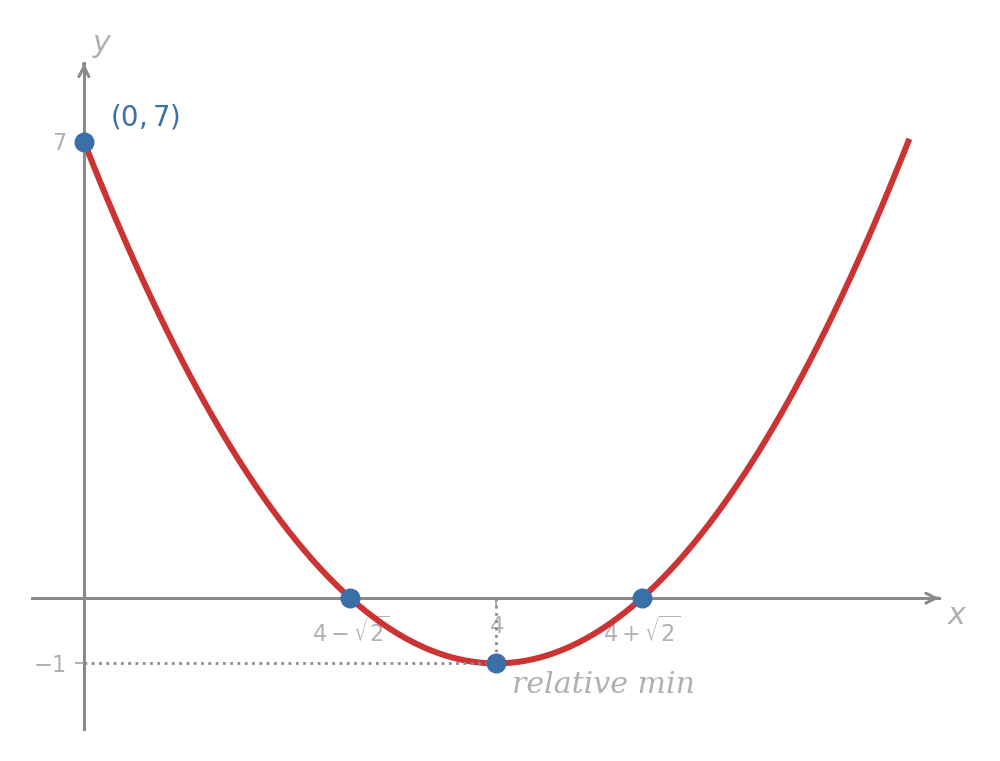
In an applied context, if this parabola modeled the height of an underwater drone over time, the $y$ -intercept would be its launch height, the minimum would be its maximum depth, and the $x$ -intercepts would be the exact moments it broke the surface of the water. This extra context turns a simple graph into a complete narrative of the drone’s journey.

Problem 90

Sketch the graph of $g(x) = -x^2 + 6x - 4$ . Find the relative extremum using either the first or the second derivative test, find the $y$ -intercept, and use the quadratic formula to find the $x$ -intercepts. What would these intercepts mean if $g(x)$ modeled the profit of a business over time?

Functions with No Critical Points

Not every function has peaks or valleys. Some processes represent unceasing growth or decay. What does the derivative tell us when a function never turns around?

Example 94 (A Function with No Critical Points)

Sketch the graph of $f(x) = \frac{1}{6}x^3 - \frac{3}{2}x^2 + 5x + 1$ .

\begin{aligned} f(x) &= \frac{1}{6}x^3 - \frac{3}{2}x^2 + 5x + 1,\\ f'(x) &= \frac{1}{2}x^2 - 3x + 5,\\ f''(x) &= x - 3. \end{aligned}

Searching for critical numbers, we set $f'(x) = 0$ and try to solve for $x$ :

\frac{1}{2}x^2 - 3x + 5 = 0.

If we apply the quadratic formula with $a = 1/2, b = -3$ , and $c = 5$ , we compute the discriminant $b^2 - 4ac = (-3)^2 - 4(1/2)(5) = 9 - 10 = -1$ . Because the discriminant is negative, there is no real solution to the equation. In other words, $f'(x)$ is never zero.

Thus, the graph cannot have relative extrema. Also, $f'(x)$ is an upward-opening quadratic with no real zeros, so since $f'(0)=5>0$ , the quadratic $f'(x)$ stays positive for every real $x$ . Therefore $f(x)$ is increasing for all $x$ .

Even though there are no extrema, we can still analyze the concavity using $f''(x)=x-3$ .

For $x < 3$ : $f''(x)$ is negative, so $f$ is concave down.
For $x = 3$ : $f''(x) = 0$ , concavity reverses.
For $x > 3$ : $f''(x)$ is positive, so $f$ is concave up.

Since $f''(x)$ changes sign at $x = 3$ , we have an inflection point at $(3, f(3)) = (3, 7)$ . The $y$ -intercept is $(0, f(0)) = (0, 1)$ . We omit the $x$ -intercept because it is difficult to solve the cubic equation $\frac{1}{6}x^3 - \frac{3}{2}x^2 + 5x + 1 = 0$ directly.

The quality of our sketch will be significantly improved if we draw the tangent line at the inflection point first. To do this, we need the slope of the graph at $(3, 7)$ :

f'(3) = \frac{1}{2}(3)^2 - 3(3) + 5 = \frac{9}{2} - 9 + 5 = \frac{1}{2}.

We draw a line through $(3, 7)$ with slope $1/2$ and then complete the curve by smoothly transitioning from concave down to concave up through that point.

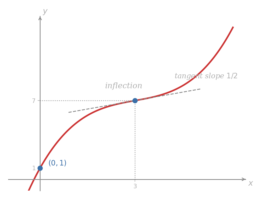
A cubic curve that constantly rises. It passes through (0,1), transitions from concave down to concave up at the inflection point (3,7), and has a drawn tangent line there with slope 1/2.

This model represents a process that is always growing, but experiences a brief period of “fatigue” where its growth slows down (concave down), hits a minimum rate of growth at the inflection point, and then re-accelerates (concave up). This is a common pattern in economic indicators or population models where growth continues despite a temporary recession in momentum.

Problem 91

Consider the function $h(x) = x^3 + 3x + 2$ . Show that $h$ has no critical numbers and is always increasing. Find its inflection point and the slope of the tangent line there. Sketch the graph.

When the Second Derivative Test Is Inconclusive

In Lesson 3AM, we noted that the second derivative test fails when $f''(a) = 0$ . When the second derivative vanishes at a critical number, the corresponding graph point could be a relative maximum, a relative minimum, or an inflection point. In these situations, returning to the first derivative test is essential.

Example 95 (Relying on the First-Derivative Test)

Sketch the graph of $f(x) = (x - 2)^4 - 1$ .

\begin{aligned} f(x) &= (x - 2)^4 - 1,\\ f'(x) &= 4(x - 2)^3,\\ f''(x) &= 12(x - 2)^2. \end{aligned}

Clearly, $f'(x) = 0$ only if $x = 2$ . So the curve has a horizontal tangent at $(2, f(2)) = (2, -1)$ .

We attempt the second derivative test: $f''(2) = 12(0)^2 = 0$ . Since the second derivative is zero, the test is inconclusive. To determine whether $(2, -1)$ is a maximum, minimum, or neither, we must apply the first derivative test by checking the sign of $f'(x)$ around $x = 2$ .

Note that:

f'(x) = 4(x - 2)^3 \begin{cases} \text{negative} & \text{if } x < 2 \\ \text{positive} & \text{if } x > 2, \end{cases}

since the cube of a negative number is negative and the cube of a positive number is positive. Therefore, as $x$ goes from left to right in the vicinity of 2, the first derivative changes sign and goes from negative to positive. By the first derivative test, the point $(2, -1)$ is a relative minimum.

The $y$ -intercept is $(0, f(0)) = (0, 15)$ because $f(0) = (0-2)^4 - 1 = 16 - 1 = 15$ . To find the $x$ -intercepts, we set $f(x) = 0$ and solve for $x$ :

\begin{aligned} (x - 2)^4 - 1 &= 0,\\ (x - 2)^4 &= 1. \end{aligned}

Taking the fourth root of both sides gives two real solutions:

\begin{aligned} x - 2 &= 1 \quad \text{or} \quad x - 2 = -1,\\ x &= 3 \quad \text{or} \quad x = 1. \end{aligned}

The curve resembles a flattened parabola.

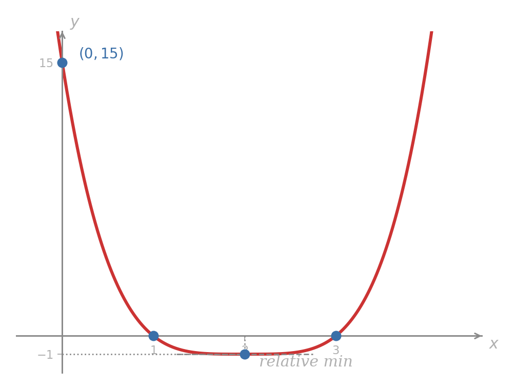
A flattened parabolic curve with a minimum at (2, -1), crossing the x-axis at 1 and 3, and the y-axis at 15.

This flat-bottomed minimum is typical of physical structures designed for stability, where small deviations from the center $x=2$ produce almost no restorative force initially (because $f''(2)=0$ ), but larger deviations result in steep restoring forces.

Problem 92

Analyze the function $k(x) = 1 - (x + 1)^4$ . Find the critical number and corresponding point, show that the second derivative test fails, and use the first derivative test to classify the point. Find the $x$ - and $y$ -intercepts and sketch the graph. What does this shape imply about stability near $x=-1$ ?

Curves with Asymptotes

The three-step procedure from Lesson 3AM, and the edge cases above, assume the function is smooth and defined at every real $x$ . Many real functions break that assumption: they blow up near some input, or their output never levels off but instead tracks a straight line for large $x$ . The final tool we need is a way to read both kinds of behavior from the formula.

Think about the cost of running a small delivery operation. You make $x$ trips per day. Each trip adds a routing cost that grows with $x$ (more trips means longer combined routes), but your fixed daily overhead of £1 is spread across all $x$ trips, contributing only $1/x$ per trip. Total cost per trip: $f(x) = x + \tfrac{1}{x}$ .

For very small $x$ , the overhead term $1/x$ dominates because the fixed overhead is spread over very few trips. For very large $x$ , the routing cost $x$ dominates and the overhead contribution vanishes. There is a sweet spot somewhere in between, and the graph reveals it. It also reveals something structurally new: an oblique asymptote, a non-horizontal line that the graph tracks ever more closely as $x \to \infty$ .

Recall from Lesson 3AM that a vertical asymptote at $x = a$ means function values grow without bound as $x \to a$ , and a horizontal asymptote $y = L$ means $f(x) \to L$ as $x \to \pm\infty$ . An oblique asymptote is the third kind: a line $y = mx + b$ such that the graph tracks the line more and more closely as $x$ becomes very large in size. The vertical distance between the graph and the line tends to zero.

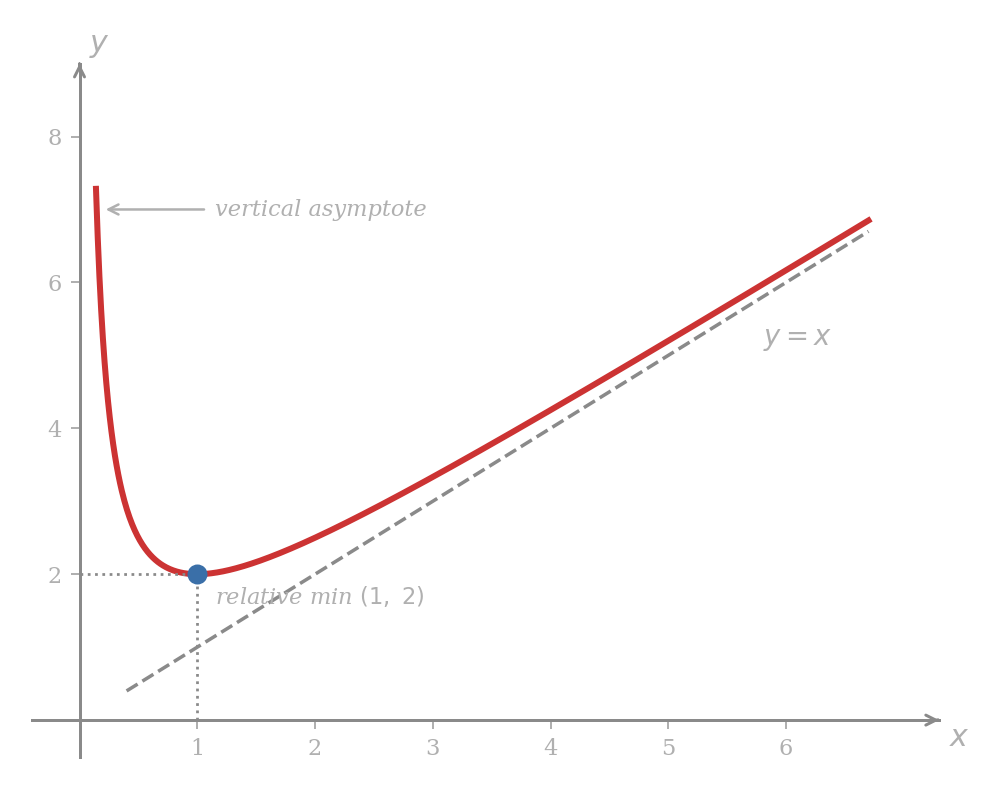
Example 96 (A Curve with a Vertical and an Oblique Asymptote)

Sketch the graph of $f(x) = x + \dfrac{1}{x}$ for $x > 0$ .

f'(x) = 1 - \frac{1}{x^2}, \qquad f''(x) = \frac{2}{x^3}.

Since $f''(x) = 2/x^3 > 0$ for all $x > 0$ , the graph is concave up throughout, so there are no inflection points. Setting $f'(x) = 0$ :

1 - \frac{1}{x^2} = 0.

This gives $x^2=1$ . Since the domain is $x>0$ , the only critical number is $x=1$ .

Since $f''(1) = 2 > 0$ , the second derivative test confirms a relative minimum at $(1, f(1)) = (1, 2)$ . Because the graph is concave up on its entire domain, this is also the absolute minimum: the lowest possible cost per trip is £2, achieved at exactly one trip per day.

Asymptotes. As $x$ shrinks toward $0$ from positive values, the term $1/x$ grows without bound, so the $y$ -axis is a vertical asymptote. For large $x$ :

f(x) - x = \frac{1}{x} \;\longrightarrow\; 0 \quad \text{as } x \to +\infty.

The line $y = x$ is an oblique asymptote: the graph lies just above $y = x$ , hugging it ever more tightly. The overhead becomes negligible and cost per trip approaches pure routing cost.

Graph of f(x) = x + 1/x for x > 0. The curve has a relative minimum at (1, 2) with dotted reference lines, approaches the y-axis as a vertical asymptote, and tracks the dashed line y = x as an oblique asymptote for large x.

An oblique asymptote is read directly from the formula when $f(x)$ splits as a linear polynomial $mx+b$ plus a term that decays to zero as $x \to \infty$ . When a function is given as a ratio of polynomials, polynomial long division separates these two pieces.

Problem 93

Consider $g(x) = x + \dfrac{4}{x}$ for $x > 0$ , which models the same delivery cost with a fixed daily overhead of £4.

Compute $g'(x)$ and $g''(x)$ .
Find the critical number, classify it using the second derivative test, and state the minimum cost per trip.
Identify the oblique asymptote. What does it represent in the delivery model?
How does this graph differ from $f(x) = x + 1/x$ ? What stays the same structurally?

The cost-minimization example in the Optimization section revisits this exact curve shape, $C(x) = 42x + 16800/x$ , with a concrete construction problem attached. The sketch above is the prototype for that calculation.

The Complete Sketching Procedure

We now have every tool needed for a full graph. Combining the three-step procedure from Lesson 3AM, the edge cases from earlier in this lesson, and the asymptote analysis above gives the complete checklist.

Note (Summary of Curve-Sketching Techniques)

Compute $f'(x)$ and $f''(x)$ .
Critical numbers. Set $f'(x) = 0$ and solve. For each critical number $a$ : compute $(a, f(a))$ , plot the point, and draw a small horizontal tangent line through it. Then apply the second derivative test: if $f''(a) > 0$ , sketch a small concave-up arc with $(a, f(a))$ as its lowest point (relative minimum); if $f''(a) < 0$ , sketch a concave-down arc with $(a, f(a))$ as its peak (relative maximum). If $f''(a) = 0$ , apply the first derivative test instead.
Inflection points. Set $f''(x) = 0$ and verify a sign change in $f''$ on each side.
Intercepts. The $y$ -intercept is $(0, f(0))$ when $0$ is in the domain. Compute $x$ -intercepts by solving $f(x) = 0$ when tractable (e.g., using the quadratic formula).
Domain restrictions. Note any excluded inputs; these produce gaps or vertical asymptotes.
Asymptotes. Evaluate $\lim_{x\to\pm\infty} f(x)$ for horizontal asymptotes. Near any excluded input $a$ , check whether $f(x) \to \pm\infty$ for a vertical asymptote. If the graph gets closer and closer to a slanted line $y = mx+b$ for very large positive or negative $x$ , that line is an oblique asymptote.

Problem 94

Sketch the graph of $h(x) = \dfrac{x^2}{x - 1}$ for $x \neq 1$ .

Carry out the full procedure: compute $h'$ and $h''$ , find the critical numbers and classify the corresponding points, identify the oblique asymptote by writing $h(x) = x + 1 + \dfrac{1}{x-1}$ , and mark the vertical asymptote at $x = 1$ .

Optimization Problems

Everything in this chapter, derivative tests, sign charts, and the full sketching procedure, was machinery in service of this section. An optimization problem asks: which value of the input makes some quantity as large or as small as possible?

The calculus is what we already know: write the function, find where $f' = 0$ , classify. The challenge in applied problems is building the function in the first place. Almost every optimization problem involves two ingredients:

an objective equation, expressing the quantity $Q$ to be optimized in terms of the available variables;
a constraint equation, a relationship the variables must satisfy.

The constraint eliminates all but one variable from the objective, producing the one-variable function whose critical numbers give the candidate answers.

The first two examples below are warm-ups where the function is handed to us directly. The remaining three require setting it up from scratch.

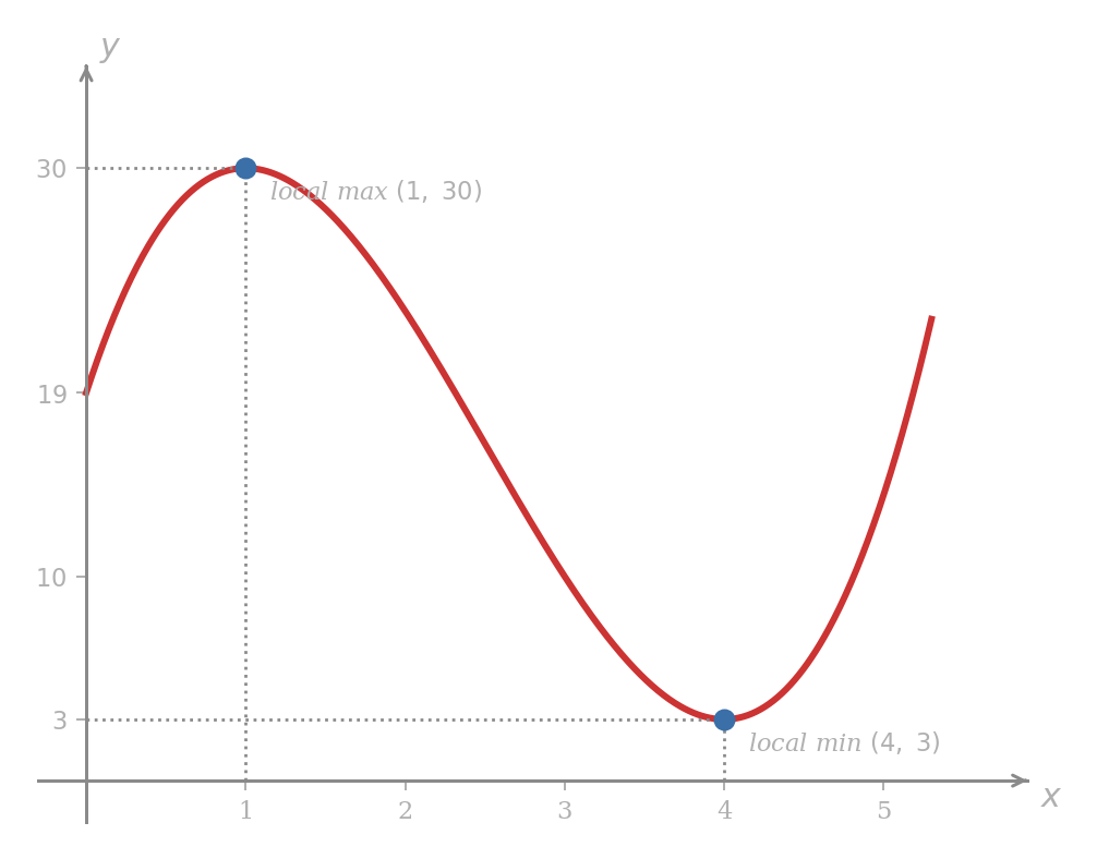
Example 97 (Minimizing a Cost Function on a Restricted Domain)

A firm’s daily production cost (in hundreds of pounds) is modeled by

f(x) = 2x^3 - 15x^2 + 24x + 19, \qquad x \geq 0,

where $x$ is thousands of units produced. Find the production level that minimizes cost.

f'(x) = 6x^2 - 30x + 24 = 6(x - 1)(x - 4), \qquad f''(x) = 12x - 30.

Critical numbers: $x = 1$ and $x = 4$ . Values:

f(1) = 2 - 15 + 24 + 19 = 30, \qquad f(4) = 128 - 240 + 96 + 19 = 3.

Second derivative test:

f''(1) = -18 < 0,

so there is a local maximum at $(1,30)$ .

f''(4) = 18 > 0,

so there is a local minimum at $(4,3)$ .

The endpoint value is $f(0)=19$ , and for large $x$ the positive cubic term forces $f(x)$ upward. Thus the local minimum at $x=4$ is the absolute minimum on the restricted domain $x \geq 0$ .

The minimum cost on $x \geq 0$ is £300, achieved at $x = 4$ thousand units per day.

Graph of f(x) = 2x³ − 15x² + 24x + 19 for x ≥ 0. A local maximum is marked at (1, 30) and a local minimum at (4, 3), each with dotted reference lines to both axes.

Problem 95

For $f(x) = 2x^3 - 15x^2 + 24x + 19$ :

Find the inflection point and confirm the concavity change on each side.
On which interval is $f$ simultaneously decreasing and concave up? What does this phase mean economically: is the cost improving, and is the improvement accelerating or slowing?
Evaluate $f(0)$ and $f(6)$ . Comparing these with the critical values, what is the global minimum of $f$ on $[0, 6]$ ?

Example 98 (Maximum Height of a Projectile)

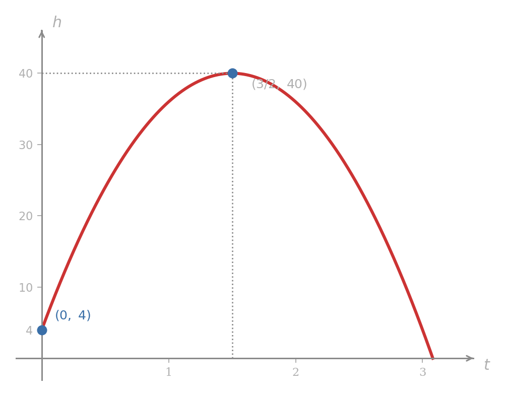
A ball is thrown vertically from a platform so that its height after $t$ seconds is

h(t) = 4 + 48t - 16t^2 \text{ feet.}

How long does it take to reach maximum height, and what is that height?

Since the coefficient of $t^2$ is negative, $h(t)$ is a downward-opening parabola with a single global maximum. Setting $h'(t) = 0$ :

48 - 32t = 0,

so $t = \frac{3}{2}$ . Since $h''(t) = -32 < 0$ , the second derivative test confirms a maximum. The maximum height is

h\!\left(\tfrac{3}{2}\right) = 4 + 72 - 36 = 40 \text{ feet.}

The ball reaches its maximum height of 40 feet at 1.5 seconds. The graph below is height as a function of time, not a picture of the physical path, which is a vertical line.

Graph of h(t) = 4 + 48t − 16t². The parabola peaks at (3/2, 40) with dotted reference lines. The h-intercept is labelled at (0, 4).

Problem 96

For $h(t) = 4 + 48t - 16t^2$ :

Use the quadratic formula to find both $t$ -intercepts. What does each root represent physically? One root is negative; does it belong to the model?
A second ball is launched from the ground with the same initial speed: $\tilde{h}(t) = 48t - 16t^2$ . At what time does it peak, and what is its maximum height? Why does it peak at the same time but lower?

The next three examples each require building the objective function from a description. That is the central skill.

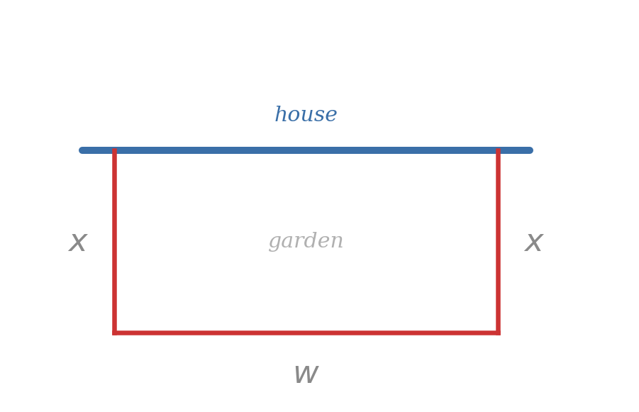
Example 99 (Maximizing the Area of a Garden)

You want to plant a rectangular garden along one side of a house, fencing the other three sides. Find the dimensions of the largest garden that can be enclosed with 40 feet of fencing.

Before setting up the general case, notice that 40 feet of fencing can be arranged in many different ways. For instance: a plot $10$ ft deep and $20$ ft wide uses $2(10)+20=40$ ft and encloses $200$ sq ft; a plot $16$ ft deep and $8$ ft wide encloses only $128$ sq ft; a plot $5$ ft deep and $30$ ft wide encloses only $150$ sq ft. The enclosed area is not fixed; it depends heavily on the choice of dimensions. Calculus will tell us exactly which choice is best.

Let $x$ be the depth (perpendicular to the house) and $w$ be the width (parallel to the house).

Objective: maximize the area,

A = wx. \tag{1}

Constraint: the fencing totals 40 feet,

2x + w = 40. \tag{2}

Solving $(2)$ for $w = 40 - 2x$ and substituting into $(1)$ :

A(x) = (40 - 2x)\,x = 40x - 2x^2, \qquad 0 \leq x \leq 20.

Setting $A'(x) = 40 - 4x = 0$ gives $x = 10$ . Since $A''(x) = -4 < 0$ everywhere, the parabola is concave down and this is an absolute maximum. From $(2)$ : $w = 20$ .

The garden of maximum area measures $x = 10$ ft deep and $w = 20$ ft wide.

Diagram of the rectangular garden. The house occupies the top edge. The three fenced sides are the bottom (width w) and both vertical sides (depth x each).

Graph of A(x) = 40x − 2x², a downward-opening parabola on [0, 20]. The maximum is at (10, 200) with dotted reference lines.

Equation $(1)$ is the objective equation; equation $(2)$ is the constraint equation. This two-equation structure is the template for every optimization problem that follows.

Problem 97

You have 60 feet of fencing for a rectangular plot against the same house wall.

Write the objective and constraint equations using the same variable names.
Express the area as a function of $x$ alone and state the domain.
Find the dimensions that maximize the enclosed area and compute that maximum.

Example 100 (Minimizing Construction Cost)

A storage yard needs a 600-square-foot rectangular enclosure. Three sides will be redwood fencing at £14 per running foot; the fourth side will be a cement wall at £28 per running foot. Find the dimensions that minimize total cost.

Let $x$ be the length of the cement side and $y$ be the length of an adjacent side.

Objective:

C = 14(x + 2y) + 28x = 42x + 28y. \tag{3}

Constraint:

xy = 600, \qquad \text{so} \qquad y = \frac{600}{x}. \tag{4}

Substituting $(4)$ into $(3)$ :

C(x) = 42x + \frac{16\,800}{x}, \qquad x > 0.

This is the same structural shape as the asymptote example: a linear term plus a reciprocal term, concave up on all of $x > 0$ , with a single minimum inside the allowed range. Setting $C'(x) = 0$ :

\begin{aligned} 42 - \frac{16\,800}{x^2} &= 0,\\ x^2 &= 400. \end{aligned}

Since $x>0$ , we get $x=20$ . Since $C''(x) = 33\,600/x^3 > 0$ , the second derivative test confirms a minimum. From $(4)$ : $y = 30$ .

Minimum cost: $C(20) = 840 + 840 = \pounds 1\,680$ . Optimal dimensions: $x = 20$ ft, $y = 30$ ft.

Graph of C(x) = 42x + 16800/x for x > 0. The curve has a minimum at (20, 1680) with dotted reference lines.

Remark

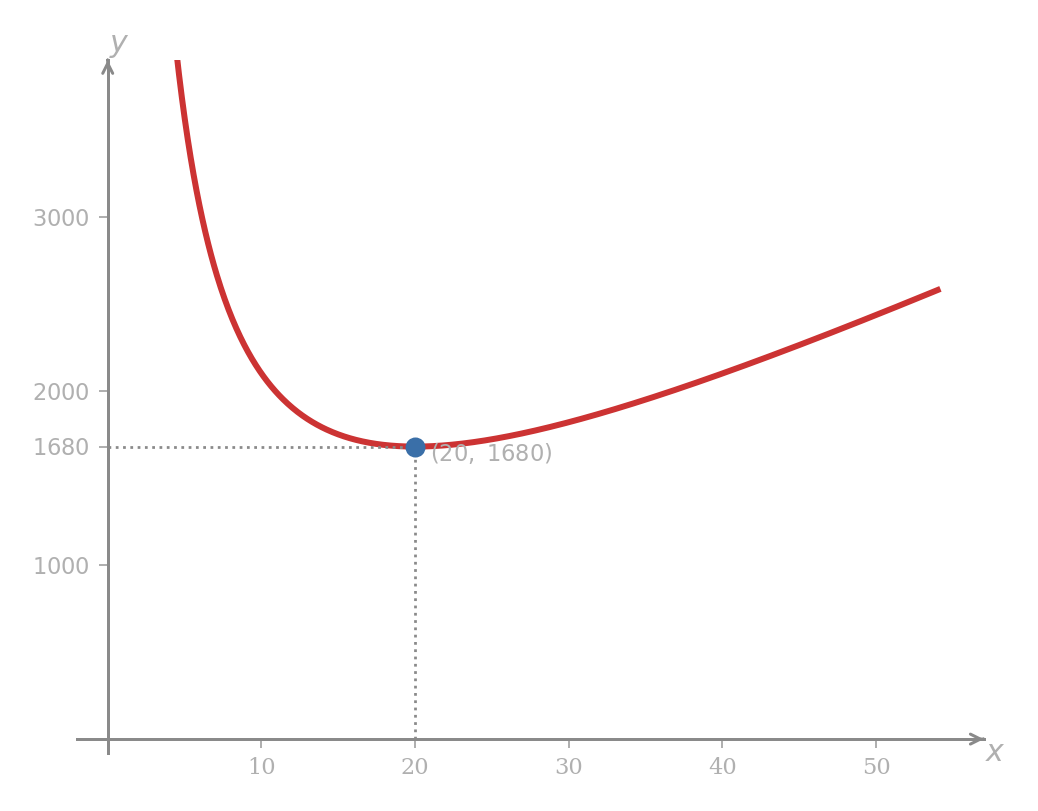
The cost function $C(x) = 42x + 16800/x$ is structurally identical to the delivery model $f(x) = x + 1/x$ : concave up everywhere, blowing up near $x = 0$ , linear for large $x$ , single minimum inside the allowed range. Recognizing this family means the minimum always satisfies $C'(x) = 0$ , turning a messy-looking cost problem into a routine derivative calculation.

Problem 98

A farmer encloses a rectangular pen of area 400 square meters against a barn wall (no fencing on the barn side). Two parallel sides cost £12 per meter; the front side costs £20 per meter.

Let $x$ be the length of the front side and $y$ be the depth. Write $C(x)$ .
Find the dimensions that minimize cost.
Confirm the minimum with the second derivative test.

Example 101 (Maximizing the Volume of a Mailable Package)

Postal regulations state that the length plus girth of a parcel may not exceed 84 inches. Find the dimensions of the cylindrical package of greatest volume satisfying this rule.

Let $l$ be the length and $r$ the radius of the circular cross-section.

Objective:

V = \pi r^2 l. \tag{5}

Constraint: the girth of a cylinder is the circumference $2\pi r$ , so

l + 2\pi r = 84, \qquad \text{so} \qquad l = 84 - 2\pi r. \tag{6}

Substituting $(6)$ into $(5)$ :

V(r) = \pi r^2(84 - 2\pi r) = 84\pi r^2 - 2\pi^2 r^3, \qquad 0 < r < \frac{42}{\pi}.

Setting $V'(r) = 0$ :

168\pi r - 6\pi^2 r^2 = 6\pi r(28 - \pi r) = 0.

The endpoint $r=0$ gives zero volume, so the useful critical number comes from $28-\pi r=0$ , namely $r=\frac{28}{\pi}$ .

Since $V''\!\left(28/\pi\right) = 168\pi - 12\pi^2\cdot(28/\pi) = 168\pi - 336\pi = -168\pi < 0$ , the second derivative test confirms a maximum. From $(6)$ : $l = 84 - 56 = 28$ inches.

The optimal package has radius $28/\pi \approx 8.9$ inches and length 28 inches.

Graph of V(r) = 84πr² − 2π²r³ for r ∈ [0, 42/π]. The volume is zero at both endpoints and peaks at r = 28/π with dotted reference lines.

Problem 99

The postal authority changes the constraint to 108 inches of length plus girth.

Write $V(r)$ under the new constraint.
Find the radius and length of the largest mailable cylinder.
Does the ratio $l : 2\pi r$ (length to girth) stay the same as under the 84-inch constraint? What does this suggest about the general shape of the optimal cylinder?

Note (Steps for Solving an Optimization Problem)

Draw a diagram where geometry is involved.
Identify the quantity $Q$ to be maximized or minimized.
Assign variable names to the quantities that may vary.
Write the objective equation: $Q$ as a function of those variables.
Write the constraint equation: the relationship the variables must satisfy.
Use the constraint to reduce the objective to a function of one variable. State the domain.
Find the critical numbers by solving $Q' = 0$ and by recording any inputs where $Q'$ does not exist while $Q$ is defined. If the domain has endpoints, check those too. Classify using the second derivative test where it applies, otherwise use the first derivative test. Compare all candidate values when needed, and answer in terms of the original problem.

Problem 100

A 12-inch square sheet of cardboard is used to make an open-top box by cutting equal squares of side $x$ from each corner and folding up the sides.

Write the volume $V(x)$ of the resulting box.
State the domain of $V$ .
Find the value of $x$ that maximizes $V$ and compute the maximum volume.

Problem 101

A manufacturer wants to produce a closed cylindrical tin holding exactly 500 cubic centimeters. Material cost is uniform per square centimeter across the curved side and both circular ends. Find the radius $r$ and height $h$ that minimize the total surface area, and verify with the second derivative test.

Note (Common Geometric Formulas for Optimization)

Shape	Formula
Rectangle	Area $= xy$ , Perimeter $= 2x + 2y$
Box	Volume $= xyz$
Circle	Area $= \pi r^2$ , Circumference $= 2\pi r$
Cylinder	Volume $= \pi r^2 h$