27/02/2026

#Math#Differentiation

Lesson assets

No linked assets.

Further Optimization Problems

Lesson 3PM fixed the two-equation template, an objective equation and a constraint equation, against geometric and physical problems: the garden against a wall, the minimum-cost enclosure, the mailable cylinder. The same template carries directly into stockrooms, into lung physiology, into the budget for advertising. Calculus changes nothing in the procedure; only the meaning of the symbols moves. The structural wrinkle this recitation forces into view is bounded domains. When the variable is confined to a closed interval, a critical number inside the interval gives only a local extremum, and the absolute optimum can sit at an endpoint instead.

Inventory Control

A retailer who orders an entire year’s stock in one delivery pays heavily on storage, insurance, and capital tied up in unsold goods. Splitting the year into many small deliveries reduces those carrying costs but multiplies the freight, clerical, and receiving cost paid per order. The two costs pull in opposite directions, so a derivative argument decides between them. The order size minimizing the total annual inventory cost is the economic order quantity.

The setup is best handled in two steps: first carrying cost alone, with the number of orders treated as a free integer parameter; then the total cost, with the order size treated as a continuous variable.

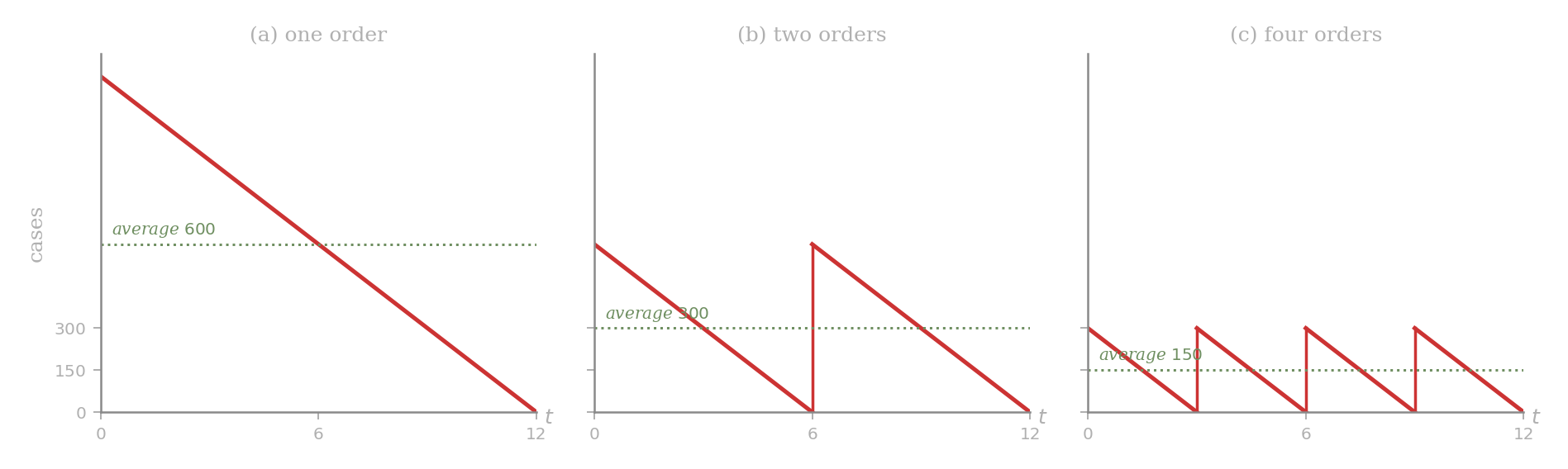
Example 1 (Carrying cost under different ordering frequencies)

A supermarket expects to sell 1200 cases of frozen orange juice at a steady rate over the next year. Carrying one case in inventory for one year costs £8, computed on the average inventory during a single order–reorder period. Equally spaced orders of equal size are placed. Find the annual carrying cost when the manager places:

one order,
two orders,
four orders.
A single delivery of 1200 cases. Inventory starts at 1200 and runs steadily down to 0, so the average inventory over the year is $\frac{1200}{2}=600$ cases. Carrying cost: $600 \times 8 = £4800$ .
Two deliveries of $1200/2 = 600$ cases each. Across each half-year the inventory drops from 600 to 0; the average is 300 cases. Carrying cost: $300 \times 8 = £2400$ .
Four deliveries of 300 cases each. The average inventory per quarter is 150 cases. Carrying cost: $150 \times 8 = £1200$ .

More frequent orders cut the carrying cost, and the cut is sizeable. Putting back a fixed cost per delivery will pull in the other direction; the optimum sits where the two marginal effects cancel.

Three sawtooth inventory graphs over a one-year horizon. Panel (a): one order of 1200 cases declining linearly to zero, average 600. Panel (b): two orders of 600 cases each, average 300. Panel (c): four orders of 300 cases each, average 150. A dotted horizontal line in each panel marks the average inventory level.

Example 2 (The economic order quantity)

For the same 1200 cases per year, each delivery now incurs an ordering cost of £75, while the carrying cost is £8 per case per year as before. Find the order size $x$ minimizing the total annual inventory cost.

Let $x$ be the order quantity in cases and $r$ the number of orders placed during the year.

Objective equation. The annual inventory cost $C$ is ordering cost plus carrying cost:

C = 75 r + 8 \!\left(\frac{x}{2}\right) = 75 r + 4x,

because the inventory of a single order–reorder period averages $x/2$ cases, and that pattern repeats unchanged across the year.

Constraint equation. The $r$ orders of size $x$ must supply the full 1200 cases:

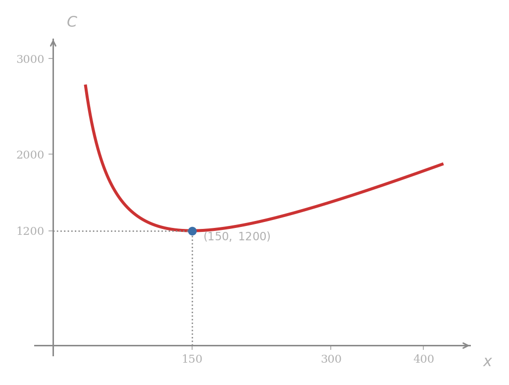
r x = 1200, \qquad \text{so} \qquad r = \frac{1200}{x}.

Substituting the constraint into the objective,

C(x) = 75 \cdot \frac{1200}{x} + 4x = \frac{90{,}000}{x} + 4x, \qquad x > 0.

The cost function is a constant times $1/x$ plus a linear term, the same structural family as the delivery cost $f(x) = x + 1/x$ from Lesson 3PM. Differentiate:

C'(x) = -\frac{90{,}000}{x^{2}} + 4.

Setting $C'(x) = 0$ ,

\begin{aligned} \frac{90{,}000}{x^{2}} &= 4,\\ x^{2} &= 22{,}500. \end{aligned}

Since $x$ is an order quantity, $x > 0$ , so $x = 150$ . The second derivative $C''(x) = 180{,}000 / x^{3} > 0$ confirms a minimum. The economic order quantity is 150 cases per order, and the corresponding number of orders is $r = 1200 / 150 = 8$ per year.

The two costs balance exactly at the optimum: ordering cost is $75 \times 8 = £600$ , carrying cost is $4 \times 150 = £600$ , total £1200. The equality is forced by $C'(x) = 0$ , not by chance.

Graph of the inventory cost function C(x) = 90000/x + 4x for x > 0. The curve carries the characteristic shape of a reciprocal plus a linear term, with a marked minimum at the point (150, 1200) and dotted reference lines projected to both axes.

Problem 1

The supermarket’s sales of frozen orange juice quadruple to 4800 cases per year, while the £75 ordering cost and the £8 per case per year carrying cost are unchanged.

Write the objective and constraint equations under the new demand.
Express $C(x)$ and compute its derivative.
Solve $C'(x) = 0$ and confirm the minimum.
Does the order quantity double, quadruple, or follow some other scaling? Read the square-root structure of the answer.

Air Velocity in a Cough

Physical models sometimes hand the objective and constraint equations across in finished form. Deriving them lies outside calculus, but once they are written the optimization proceeds unchanged.

Example 3 (Velocity of expelled air during a cough)

To clear the trachea during a cough the body raises the velocity $v$ of the expelled air by contracting the airway against an increase in pressure. Two empirical relations describe the situation. Let $r_{0}$ be the resting radius of the trachea, $r$ the radius during a cough, $P$ the increase in air pressure, and $v$ the air velocity.

(Constraint) The decrease in radius is nearly proportional to the increase in pressure: $r_{0} - r = a P$ with $a > 0$ .
(Objective) Flow theory gives $v$ proportional to the product of the pressure increase and the cross-sectional area: $v = b P \cdot \pi r^{2}$ with $b > 0$ . Absorbing the constant $\pi b$ into a single positive constant $k$ gives $v = k P r^{2}$ .

Maximise $v$ over $0 \leq r \leq r_{0}$ .

Solving the constraint for $P = (r_{0} - r) / a$ and substituting into the objective,

v(r) = \frac{k}{a}\,(r_{0} - r)\,r^{2} = \tilde{k}\,(r_{0} r^{2} - r^{3}), \qquad \tilde{k} = \frac{k}{a} > 0.

Differentiating,

v'(r) = \tilde{k}\,(2 r_{0} r - 3 r^{2}) = \tilde{k}\, r\,(2 r_{0} - 3 r).

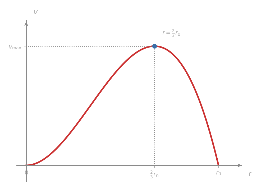
The zeros of $v'$ are $r = 0$ and $r = \tfrac{2}{3} r_{0}$ . The critical number inside the interval is the substantive candidate, the other being an endpoint. The second derivative,

v''(r) = \tilde{k}\,(2 r_{0} - 6 r),

evaluated at $r = \tfrac{2}{3} r_{0}$ gives $v''\!\bigl(\tfrac{2}{3} r_{0}\bigr) = -2 \tilde{k} r_{0} < 0$ , so that critical number gives a local maximum. The endpoint values are $v(0) = 0$ and $v(r_{0}) = 0$ , both below $v\!\bigl(\tfrac{2}{3} r_{0}\bigr) > 0$ , so the local maximum is the absolute maximum on the closed interval.

The optimal contraction during a cough is to two-thirds of the resting radius, independent of the empirical constants $a$ and $b$ . The ratio is forced by the structure of the model.

Graph of v(r) = k(r0 r squared minus r cubed) on the interval from r equals 0 to r equals r0. The curve rises from zero at the left endpoint, peaks at r equals two-thirds of r0, and returns to zero at r equals r0. The peak is marked, with dotted reference lines drawn to both axes.

Remark (The endpoint candidates were not optional)

Both ends of the interval, $r = 0$ and $r = r_{0}$ , were checked alongside the critical number inside the interval. They turned out to be tied at $v = 0$ and so could not displace the maximum, but the sample was forced rather than freely chosen: on a closed interval, any candidate for the absolute optimum that lies on the boundary must be evaluated and compared against the critical numbers. The next section makes the warning bite.

When the Optimum Sits at an Endpoint

In the inventory problem and the cough model the critical number inside the interval won outright. The next example shows the opposite outcome: the global maximum lies at an endpoint, while the critical number inside the interval gives only a local minimum. A zero of the derivative gives a candidate, no more; the trouble is that local extrema need not be the answer to the applied question.

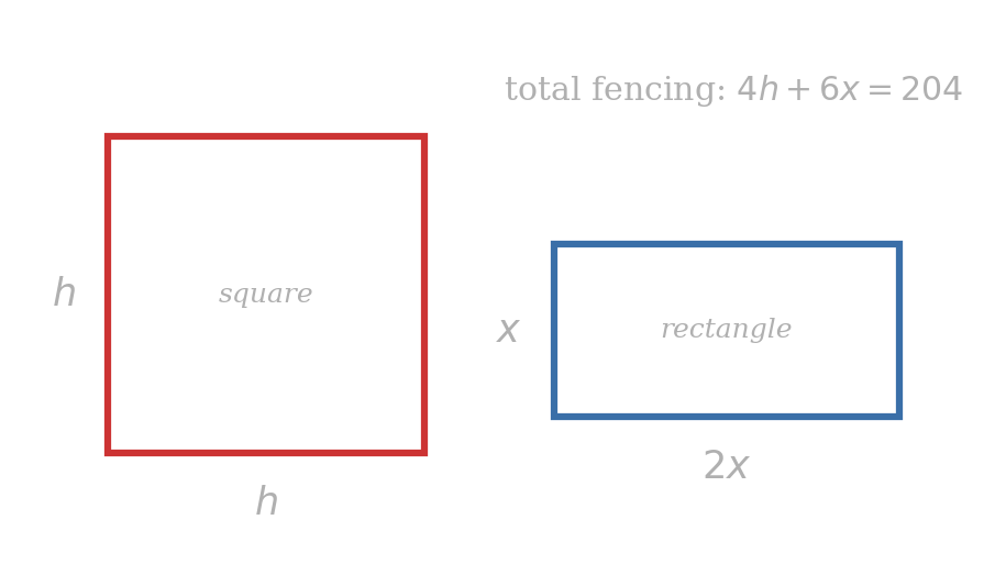
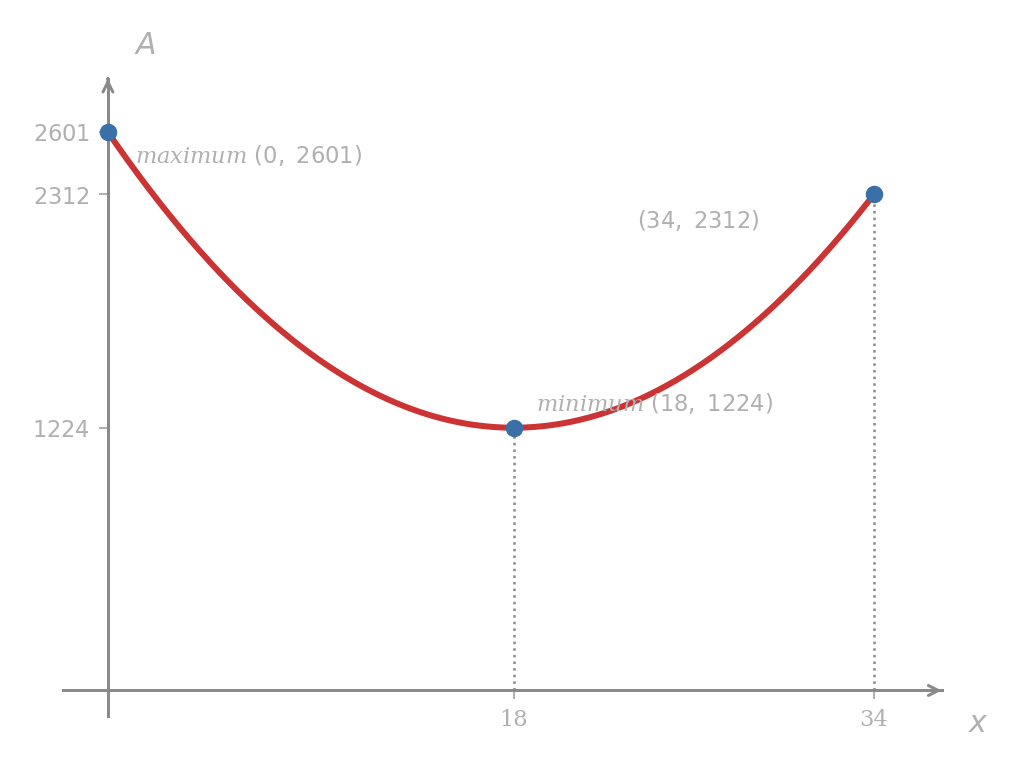
Example 4 (Maximizing the combined area of two corrals with a fixed length of fencing)

A rancher has 204 meters of fencing to enclose two separate corrals: one square, the other a rectangle whose length is twice its width. Non-negative dimensions are admissible, so either corral may degenerate to width zero. Find the dimensions giving the largest combined area.

Let $x$ be the width of the rectangle (so its length is $2x$ ) and $h$ the side length of the square.

Objective equation. The combined area is

A = h^{2} + (2x)(x) = h^{2} + 2x^{2}. \tag{1}

Constraint equation. The total fencing along the four sides of each corral is

4h + (2x + x + 2x + x) = 4h + 6x = 204. \tag{2}

The rectangle has two sides of length $2x$ and two of length $x$ , summing to $6x$ . Non-negativity of the dimensions and the fixed total give $0 \leq 6x \leq 204$ , i.e. $0 \leq x \leq 34$ .

Solving (2) for $h = \tfrac{1}{4}(204 - 6x) = 51 - \tfrac{3}{2} x$ and substituting into (1),

A(x) = \!\left(51 - \tfrac{3}{2}x\right)^{2} + 2x^{2}, \qquad 0 \leq x \leq 34.

Expanding,

\begin{aligned} A(x) &= 2601 - 153x + \tfrac{9}{4}x^{2} + 2x^{2} \\ &= 2601 - 153x + \tfrac{17}{4}x^{2}. \end{aligned}

Differentiating,

A'(x) = -153 + \tfrac{17}{2}x.

Setting $A'(x) = 0$ gives $x = 18$ . The second derivative is $A''(x) = \tfrac{17}{2} > 0$ everywhere, so the parabola is concave up and $x = 18$ supplies a local minimum of $A$ . Since the problem asks for the maximum, the answer must lie at an endpoint.

Evaluating the endpoints,

\begin{aligned} A(0) &= 2601, \\ A(34) &= 2601 - 153(34) + \tfrac{17}{4}(34)^{2} \\ &= 2601 - 5202 + 4913 = 2312. \end{aligned}

The absolute maximum on $[0, 34]$ is $A(0) = 2601$ square meters, attained at $x = 0$ . From the constraint $h = 51$ . The rancher should build only the square corral, of side 51 m, and omit the rectangle altogether. The critical number $x = 18$ gives the smallest combined area, $A(18) = 1224$ square meters.

A zero of the derivative gives a candidate, no more. The applied question may demand the opposite kind, and on a closed interval the answer can sit at the boundary while the critical number points in the wrong direction.

Diagram of the two corrals drawn separately. The square corral on the left has all four sides labeled h. The rectangular corral on the right has width x and length 2x. A heading above the figure records the total fencing constraint 4h plus 6x equals 204.

Graph of A(x) equals 2601 minus 153x plus seventeen-quarters x squared on the closed interval from 0 to 34, an upward-opening parabola. The left endpoint at (0, 2601) is the absolute maximum, the critical number x equals 18 attains the minimum value A equals 1224, and the right endpoint at (34, 2312) sits between the two. All three points are marked.

Problem 2

A farmer has 300 meters of fencing to enclose a rectangular field and divide it into two equal pens by a fence parallel to one side. Let $x$ be the length of the side perpendicular to the dividing fence.

Sketch the configuration and write the objective and constraint equations.
Express the area $A$ as a function of $x$ on a closed interval.
Find the critical number and classify it.
Identify the absolute maximum and the corresponding dimensions.

Optimal Advertising Spend

The first three sections fixed the optimum either through cost-versus-cost trade-offs or through a physical model. The next setting is closer to economic reality: a single spending decision controls revenue, and the firm chooses the spend at which net profit peaks.

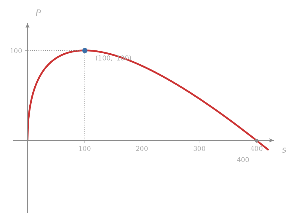
Example 5 (Profit as a function of advertising spend)

A firm estimates that the weekly gross revenue from a product, in thousands of pounds, is

R(s) = 20 \sqrt{s},

where $s$ (in thousands of pounds) is the weekly amount spent on advertising. Gross revenue here is revenue from sales before deducting advertising cost. The net weekly profit is

P(s) = R(s) - s = 20 \sqrt{s} - s, \qquad s \geq 0.

Find the spend that maximizes net profit.

Writing $P(s) = 20 s^{1/2} - s$ , the power rule and the sum rule give

P'(s) = 20 \cdot \tfrac{1}{2} s^{-1/2} - 1 = \frac{10}{\sqrt{s}} - 1.

Setting $P'(s) = 0$ ,

\begin{aligned} \frac{10}{\sqrt{s}} &= 1, \\ \sqrt{s} &= 10, \\ s &= 100. \end{aligned}

The second derivative is $P''(s) = -5 s^{-3/2} < 0$ for all $s > 0$ , so $s = 100$ supplies a local maximum. Since $P(0) = 0$ and $P(s) \to -\infty$ as $s \to \infty$ , the local maximum is also the absolute maximum on $s \geq 0$ . The optimal weekly advertising spend is £100,000, generating a net profit of $20(10) - 100 = 100$ thousand pounds, or £100,000. Spending less than £100k leaves revenue on the table; spending more buys revenue at a worse rate than the cost of buying it.

Graph of P(s) equals 20 root s minus s for s between 0 and roughly 400. The curve rises from the origin, peaks at the point (100, 100), and then declines, passing through zero again at s equals 400. The maximum point is marked with dotted reference lines projected to both axes.

Problem 3

The firm revises its revenue model to $R(s) = 30 s^{2/3}$ (in thousands of pounds) for the same weekly advertising spend $s$ .

Write the new net profit function $P(s)$ .
Find the spend maximizing net profit.
Confirm with the second derivative test.
Compare the optimum with that of the square-root model. Which model prescribes the more aggressive spend, and why does the comparison run that way?

Cost, Revenue, and Profit

Optimization in business and economics rests on three functions of a single variable, the production level $x$ :

the cost function $C(x)$ , the cost of producing $x$ units;
the revenue function $R(x)$ , the revenue from selling $x$ units;
the profit function $P(x) = R(x) - C(x)$ , the difference between the two.

Strictly $x$ takes only non-negative integer values, since fractional cars and refrigerators are never sold, but for the purposes of differentiation each function is interpolated to a smooth curve over $x \geq 0$ . Answers are then read in light of the original integer setting whenever that interpretation matters.

The derivatives $C'(x)$ , $R'(x)$ , and $P'(x)$ are called marginal cost, marginal revenue, and marginal profit, respectively. Each measures the rate at which the corresponding total responds to one more unit produced. Calculus reduces every question in this section to the location of zeros of one of these marginal functions.

Marginal Cost

A typical cost function is concave down for small $x$ and concave up for large $x$ . The shape encodes two opposing forces. At low production levels the firm benefits from economies of scale, fixed overhead spread over more output, bulk-rate inputs, so each additional unit is cheaper than the last; the cost rises but at a slowing rate. At high production levels the firm hits overtime, less efficient plant, and competition for scarce inputs, so each additional unit is more expensive than the last. The transition between the two regimes is exactly where the marginal cost is least.

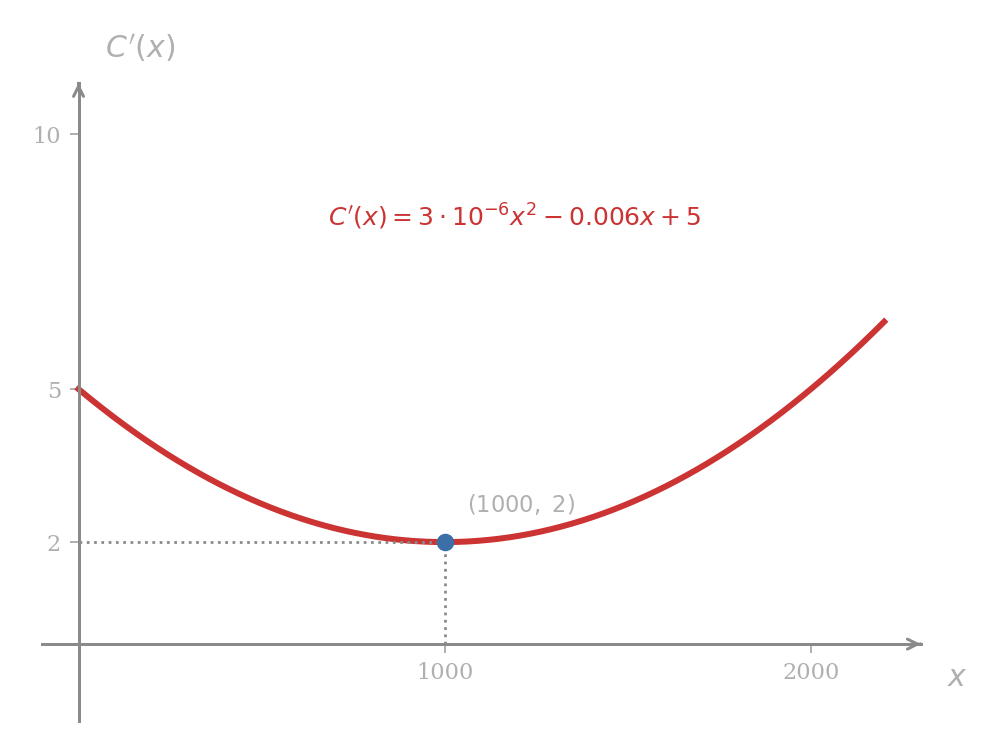
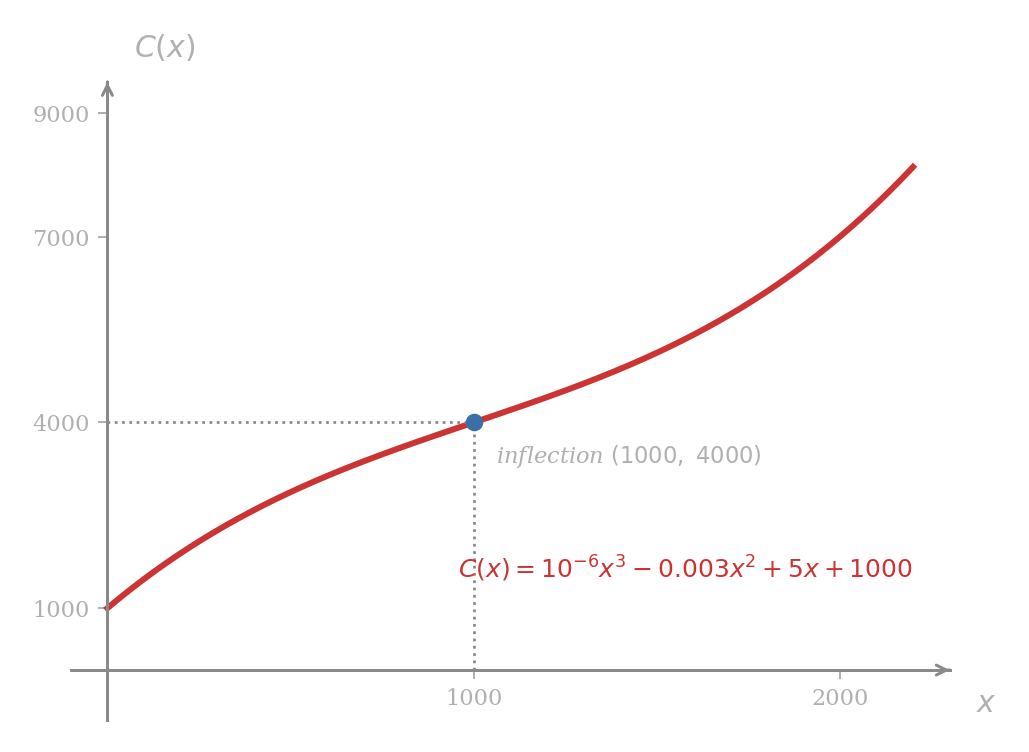
Example 6 (Locating the inflection point of a cost function)

A manufacturer’s daily cost (in pounds) is

C(x) = 10^{-6} x^{3} - 0.003 x^{2} + 5 x + 1000.

Describe the behavior of the marginal cost and sketch $C(x)$ .

Differentiating,

\begin{aligned} C'(x) &= 3 \cdot 10^{-6} x^{2} - 0.006 x + 5, \\ C''(x) &= 6 \cdot 10^{-6} x - 0.006 = 6 \cdot 10^{-6} (x - 1000). \end{aligned}

The marginal cost $C'(x)$ is itself a parabola opening upwards, with $\bigl(C'\bigr)'\!(x) = C''(x)$ vanishing at $x = 1000$ . So $C'(x)$ has its minimum at $x = 1000$ , with value

C'(1000) = 3 \cdot 10^{-6}(10^{6}) - 0.006(1000) + 5 = 3 - 6 + 5 = 2.

Marginal cost decreases for $x < 1000$ , attains its minimum of £2 per unit at the production level $x = 1000$ , and increases thereafter.

The graph of $C(x)$ is now read off from $C'(x)$ . Since $C'(x) > 0$ for every $x \geq 0$ , the cost is increasing throughout, as any cost ought to be. The sign of $C''(x) = 6 \cdot 10^{-6}(x - 1000)$ flips at $x = 1000$ : $C$ is concave down on $(0, 1000)$ and concave up on $(1000, \infty)$ , so $x = 1000$ is an inflection point of the cost curve. The inflection of $C$ sits exactly above the minimum of $C'$ , the point at which the firm switches from economies of scale to diseconomies of scale.

Graph of the marginal cost C prime of x equals 3 times ten to the minus six x squared minus 0.006 x plus 5, an upward-opening parabola. The minimum is marked at the point (1000, 2) with dotted reference lines projected to both axes. The curve sits entirely above the x-axis.

Graph of the cost function C of x corresponding to the cubic above, plotted for x from 0 to roughly 2000. The curve rises throughout, is concave down on the interval from 0 to 1000, and turns concave up beyond 1000. The inflection point at x equals 1000 is marked with a dotted vertical reference line, lining up directly above the minimum of the marginal-cost parabola.

Revenue and the Demand Equation

When a firm faces many competitors, its own sales barely move the market price, so $R(x) = p x$ for a constant $p$ and the revenue curve is a straight line through the origin. The interesting case is the monopolist, the only supplier of the product. Customers buy more units at a low price and fewer at a high price, so for each quantity $x$ there is a highest price $p = f(x)$ at which all $x$ units can be sold. The function $f$ is decreasing; its graph is the demand curve. Total revenue is then

R(x) = x \cdot p = x \cdot f(x),

no longer a straight line but typically a downward-opening curve with a maximum.

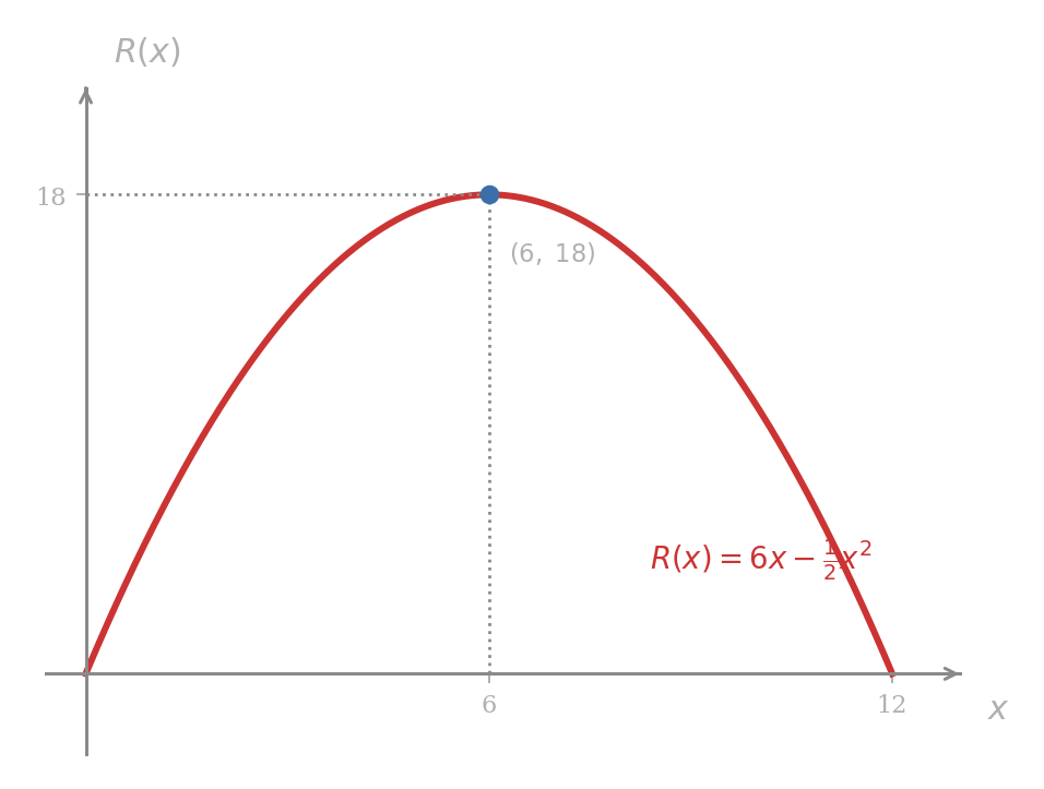
Example 7 (Maximizing revenue under a linear demand curve)

The demand equation for a monopolist’s product is $p = 6 - \tfrac{1}{2} x$ pounds. Find the production level giving the greatest total revenue.

Total revenue is

R(x) = x \!\left(6 - \tfrac{1}{2} x\right) = 6 x - \tfrac{1}{2} x^{2},

a downward-opening parabola. The marginal revenue is $R'(x) = 6 - x$ , which vanishes at $x = 6$ . Since $R''(x) = -1 < 0$ , the critical number gives the absolute maximum. The corresponding revenue is

R(6) = 6(6) - \tfrac{1}{2}(36) = 36 - 18 = 18 \text{ pounds}.

Selling 6 units at $p = 6 - \tfrac{1}{2}(6) = 3$ pounds each maximizes revenue at £18.

Graph of the revenue function R of x equals 6x minus one half x squared, a downward-opening parabola. The maximum is marked at the point (6, 18) with dotted reference lines projected to both axes.

The demand equation is rarely handed across in finished form. More often the firm has only a handful of price-quantity observations and must fit a curve, the simplest choice being a straight line through two known points.

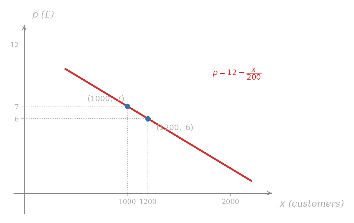
Example 8 (Setting up a linear demand equation from data)

An open-top tour bus operator priced its city circuit at £7 per ticket and averaged 1000 customers per week. After the price was lowered to £6, weekly demand rose to 1200. Assuming the demand equation is linear, find the ticket price that maximizes weekly revenue.

The two points $(x, p) = (1000, 7)$ and $(1200, 6)$ lie on the demand line. Its slope is

\frac{6 - 7}{1200 - 1000} = -\frac{1}{200}.

Using the point-slope form anchored at $(1000, 7)$ ,

p - 7 = -\frac{1}{200}(x - 1000), \qquad \text{so} \qquad p = 12 - \frac{x}{200}.

Total revenue is

R(x) = x \!\left(12 - \frac{x}{200}\right) = 12 x - \frac{x^{2}}{200}.

The marginal revenue is

R'(x) = 12 - \frac{x}{100}.

Setting $R'(x) = 0$ gives $x = 1200$ . Since $R''(x) = -\tfrac{1}{100} < 0$ , the critical number maximizes revenue. The corresponding price is

p = 12 - \frac{1200}{200} = 12 - 6 = £6,

and the maximum weekly revenue is

R(1200) = 12(1200) - \frac{1200^{2}}{200} = 14{,}400 - 7200 = £7200.

Of the two prices already tested, the £6 price was already at the optimum; the £7 price was leaving £200 a week on the table.

Demand line drawn on the price-quantity plane. The horizontal axis is customers per week, the vertical axis is ticket price in pounds. Two anchor points are marked at (1000, 7) and (1200, 6), with the line passing through both and extended in either direction. Dotted reference lines drop from each anchor to the axis.

Maximizing Profit

With the cost function and the revenue function in hand, the profit function $P(x) = R(x) - C(x)$ is differentiated like any other; the critical number gives the optimum production level whenever the second derivative test confirms a maximum.

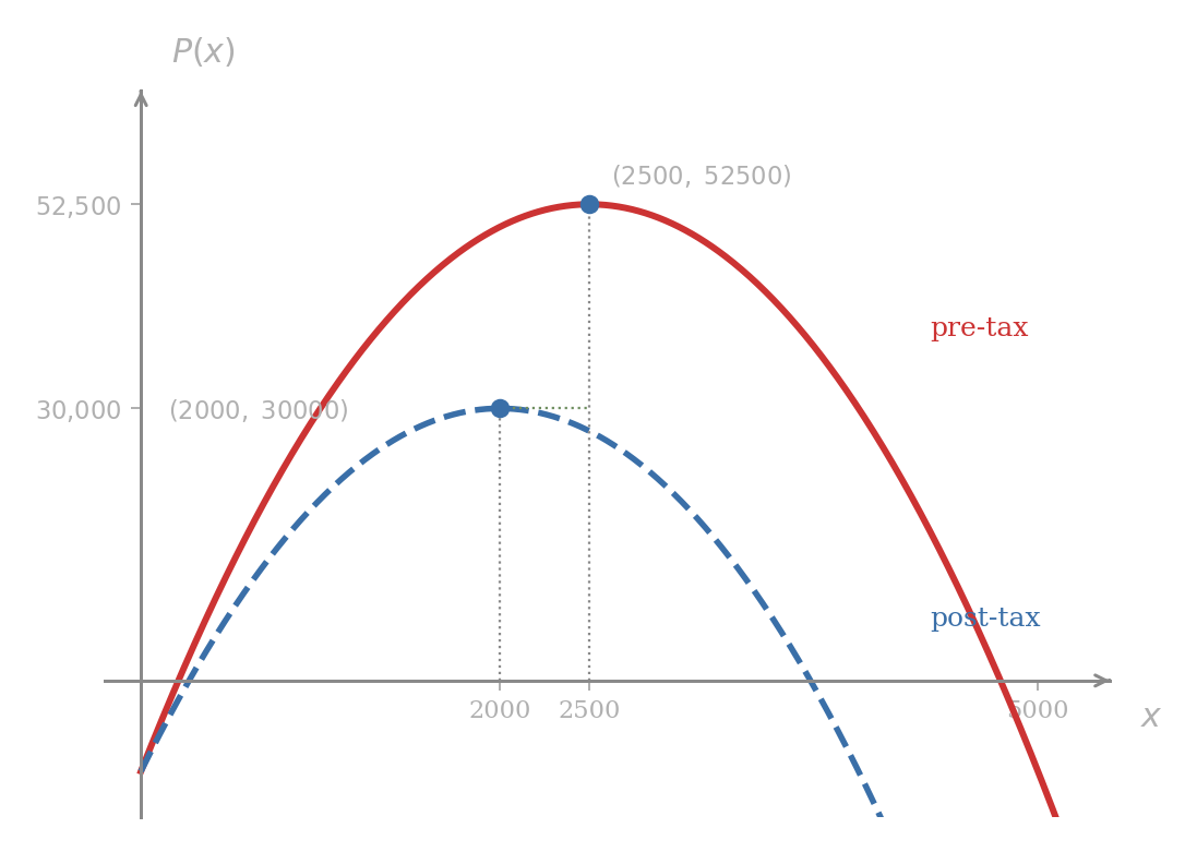
Example 9 (Maximizing profit for a monopolist)

The demand equation for a monopolist is $p = 100 - 0.01 x$ pounds, and the cost function is $C(x) = 50 x + 10{,}000$ pounds. Find the production level maximizing profit, the corresponding price, and the maximum profit.

Total revenue is

R(x) = x (100 - 0.01 x) = 100 x - 0.01 x^{2},

so the profit function is

P(x) = R(x) - C(x) = 100 x - 0.01 x^{2} - (50 x + 10{,}000) = -0.01 x^{2} + 50 x - 10{,}000.

The graph of $P$ is a downward-opening parabola. Its marginal profit is

P'(x) = -0.02 x + 50 = -0.02 (x - 2500),

so $P'(x) = 0$ at $x = 2500$ . The second derivative $P''(x) = -0.02 < 0$ confirms a maximum. The maximum profit is

P(2500) = -0.01(2500)^{2} + 50(2500) - 10{,}000 = -62{,}500 + 125{,}000 - 10{,}000 = £52{,}500.

The price the monopolist should charge to clear all 2500 units is

p = 100 - 0.01(2500) = 100 - 25 = £75.

Producing 2500 units at £75 each yields a profit of £52,500.

Profit Under an Excise Tax

A tax levied per unit produced is absorbed cleanly into the cost function, leaving the demand equation untouched. The shape of the analysis is identical; only the constants move.

Example 10 (The same monopolist after a £10 excise tax)

The government imposes an excise tax of £10 per unit. Repeat the previous example.

Each unit sold now carries an additional £10 cost paid to the government, so the cost function becomes

C(x) = (50 x + 10{,}000) + 10 x = 60 x + 10{,}000.

The demand equation, and so the revenue function, is unchanged: $R(x) = 100 x - 0.01 x^{2}$ . The new profit function is

\begin{aligned} P(x) &= R(x) - C(x) \\ &= 100 x - 0.01 x^{2} - (60 x + 10{,}000) \\ &= -0.01 x^{2} + 40 x - 10{,}000. \end{aligned}

The marginal profit is

P'(x) = -0.02 x + 40 = -0.02 (x - 2000),

so $P'(x) = 0$ at $x = 2000$ . The second derivative $P''(x) = -0.02 < 0$ confirms a maximum. The new maximum profit is

P(2000) = -0.01(2000)^{2} + 40(2000) - 10{,}000 = -40{,}000 + 80{,}000 - 10{,}000 = £30{,}000,

and the new price is

p = 100 - 0.01(2000) = £80.

The optimal price has risen from £75 to £80, but only by half the £10 tax. The monopolist passes half the tax onto the consumer and absorbs the other half in reduced margin; the profit collapses from £52,500 to £30,000. No production decision can recover the lost £22,500. The drop is the structural reason firms lobby against per-unit taxation.

Two profit parabolas drawn on the same axes. The pre-tax profit P of x equals minus 0.01 x squared plus 50x minus ten thousand peaks at the point (2500, 52500). The post-tax profit P of x equals minus 0.01 x squared plus 40x minus ten thousand sits below it and peaks at the point (2000, 30000). Both peaks are marked, and a thin dotted segment connects them to highlight the leftward and downward shift caused by the tax.

Note (Marginal revenue equals marginal cost at the optimum)

At a production level $x = a$ that maximizes profit, $P'(a) = 0$ , and since $P = R - C$ the equation reads

R'(a) = C'(a).

Profit is maximized at the production level where marginal revenue equals marginal cost. The principle is the structural lesson of the section, separate from any particular cost or demand model.

Problem 4

A firm has cost function $C(x) = 0.002 x^{3} - 0.6 x^{2} + 75 x + 100$ and faces the demand equation $p = 200 - x$ .

Write the revenue function $R(x)$ and the profit function $P(x)$ .
Compute $R'(x)$ , $C'(x)$ , and the critical number satisfying $R'(x) = C'(x)$ .
Confirm with the second derivative test that the critical number maximizes $P$ .
Compute the optimal price and the maximum profit.

Exercises

Exercise 1

A small retailer sells 800 units of a product per year at a constant rate. The ordering cost is £40 per order and the carrying cost is £5 per unit per year. Find the economic order quantity and the minimum annual inventory cost.

Exercise 2

For the general inventory model with annual demand $D$ , ordering cost $K$ per order, and carrying cost $h$ per unit per year, derive the closed form of the economic order quantity, $x = \sqrt{2 D K / h}$ .

Exercise 3

For the windpipe model, show that the radius maximizing the air velocity is exactly $\tfrac{2}{3}$ of the resting radius, independently of the empirical constants $a$ and $b$ . The ratio $r / r_{0}$ is a structural invariant of the model.

Exercise 4

A rectangular page is to contain 54 square inches of printed matter, with 1-inch margins at the top and bottom and 1.5-inch margins at the sides. Find the dimensions of the page that minimize the amount of paper used.

Exercise 5

The cost of running a ship at a steady speed $v$ knots is $C(v) = a v^{3} + b / v$ pounds per hour, with $a, b > 0$ . Find the speed minimizing the hourly cost, and show that at the minimizing speed the term $a v^{3}$ is exactly one-third of the term $b / v$ .

Exercise 6

Find the points on the parabola $y = x^{2}$ closest to $(0, 3)$ . Minimize the square of the distance rather than the distance itself, and justify that the answer gives the absolute minimum.

Exercise 7

A right circular cylinder is inscribed in a sphere of radius $R$ . With cylinder radius $r$ and height $h$ , the cross-section gives

r^{2} + \!\left(\frac{h}{2}\right)^{2} = R^{2}.

Find the height $h$ that maximizes the cylinder’s volume.

Exercise 8

A monopolist faces the demand equation $p = 25 - 0.02 x$ and has cost function $C(x) = 5 x + 600$ .

Find the production level maximizing profit and the corresponding price.
The government imposes an excise tax of £4 per unit. Find the new optimal production level, the new price, and the loss of profit caused by the tax.
By what fraction of the tax is the price raised?

Exercise 9

A firm’s marginal cost is $C'(x) = 3 x^{2} - 80 x + 700$ . Find the production level minimizing the marginal cost, and compute the minimum marginal cost.