18/02/2026

#Math#Differentiation

Video

Lesson assets

video link

CS50P Lecture 0: Functions, Variables

recitation

Recitation

Homework 2 PDF

Limits and Derivatives

The Derivative

Lesson 2AM attached a slope to every point of a smooth curve through the construction of its tangent line. When the curve is the graph of a function $f$ , that slope at the input $x$ is determined by $x$ alone, so it defines a new function of $x$ : the rule that sends each input to the slope of $f$ there.

Definition 22 (Derivative)

Let $f$ be a function whose graph admits a tangent line at the point $(x, f(x))$ . The derivative of $f$ at $x$ is the slope of the curve $y = f(x)$ at that point, written $f'(x)$ . The function $f'$ whose value at each such input is $f'(x)$ is itself called the derivative of $f$ , and its domain is the collection of inputs at which $f$ admits a tangent. The process of computing $f'$ from $f$ is called differentiation.

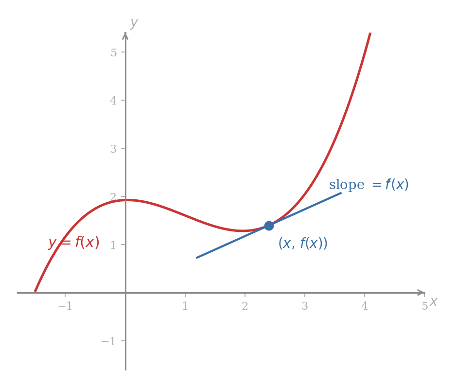
A smooth curve y equals f of x with a marked point (x, f of x) on it and the tangent line drawn at that point. The slope of the tangent line is labelled f prime of x, and the curve is shown extending in both directions to indicate that as x varies, the same construction produces a slope at every input.

The notation $f'(x)$ depends on $x$ as the original $f(x)$ does, so $f'$ is itself a function and may be evaluated, plotted, and combined exactly as $f$ was. Its domain consists of those inputs at which the curve $y = f(x)$ admits a tangent; at points of the absolute-value type singled out in Lesson 2AM, no tangent exists and $f'$ is left undefined there.

Linear and constant functions

For a linear function $f(x) = mx + b$ the graph is the line of slope $m$ . The tangent line to a line at any of its points is the line itself, since no other straight line approximates a straight line better than the line does, so the slope of the graph at every input is $m$ . The derivative is therefore the constant function with value $m$ :

\text{If } f(x) = mx + b, \text{ then } f'(x) = m.

The case $m = 0$ collapses $f$ to the constant function $f(x) = b$ , whose graph is the horizontal line at height $b$ and whose tangent at every point is that horizontal line itself, of slope $0$ . So

\text{If } f(x) = b \text{ is constant, then } f'(x) = 0.

Two side-by-side panels. The left panel shows a non-horizontal straight line of slope m drawn in the plane, with the same straight line marked again as its own tangent at a marked point on it. The right panel shows a horizontal line at height b with a horizontal tangent drawn at a marked point on it, indicating slope zero at every input.

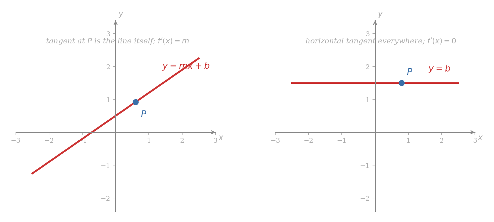
Differentiation strips a linear function down to its slope, sending the constant term to zero. The two facts will be invoked silently throughout the rest of the course.

The cases $x^2$ and $x^3$

The slope formula recorded as a Theorem in Lesson 2AM, that the slope of $y = x^2$ at the point $(a, a^2)$ is $2a$ , translates immediately into the derivative.

Note

If $f(x) = x^2$ , then $f'(x) = 2x$ .

A parallel calculation, deferred together with the slope formula above to the limit construction later in this lesson, gives the derivative of the cube.

Note

If $f(x) = x^3$ , then $f'(x) = 3x^2$ .

Comparing the two,

(x^2)' = 2 x^{2 - 1}, \qquad (x^3)' = 3 x^{3 - 1},

the exponent dropping by one and reappearing in front. The pattern extends to every power function in the sense of Lesson 1PM and supplies the most useful single rule of elementary differentiation.

The Power Rule

Theorem 4 (Power Rule)

Let $r$ be a rational number, and let $f(x) = x^r$ on the inputs at which the power is defined. Then on the inputs at which the curve $y = x^r$ admits a tangent line,

f'(x) = r\,x^{r - 1}.

The proof requires the limit construction developed later in this lesson, and the full rational-exponent case is deferred to a later MA0A lesson. The special cases $r = 1, 2, 3$ recover the linear, parabolic, and cubic results already obtained, and $r = 0$ recovers the constant-function result via $f(x) = x^0 = 1$ on $x \neq 0$ with $f'(x) = 0 \cdot x^{-1} = 0$ . The remaining rational $r$ extend the toolkit to every root and reciprocal of a root.

Example 54 (Derivative of

\sqrt{x}

)

Writing $\sqrt{x} = x^{1/2}$ as in Recitation 1, the power rule with $r = \tfrac{1}{2}$ gives

f'(x) = \tfrac{1}{2} x^{1/2 - 1} = \tfrac{1}{2} x^{-1/2} = \frac{1}{2 \sqrt{x}}.

The derivative is defined for every $x > 0$ . At $x = 0$ the original $\sqrt{x}$ is defined but the curve has a vertical tangent there, so the slope is not a real number and $f'$ is not defined at the origin.

Example 55 (Derivative of

1/x

)

Writing $1/x = x^{-1}$ , the power rule with $r = -1$ gives

f'(x) = (-1) \, x^{-1 - 1} = -x^{-2} = -\frac{1}{x^2}.

The derivative is defined for every $x \neq 0$ , the same restriction $1/x$ itself carries.

Example 56 (Derivative of

x^{2/3}

)

The power rule with $r = \tfrac{2}{3}$ gives

f'(x) = \tfrac{2}{3} x^{2/3 - 1} = \tfrac{2}{3} x^{-1/3} = \frac{2}{3\, x^{1/3}}.

The original $x^{2/3}$ is defined on every real $x$ , since $\tfrac{2}{3}$ has odd denominator, but the curve has a vertical tangent at the origin and so $f'$ excludes $x = 0$ .

Problem 35

Use the power rule to compute $f'(x)$ for each of the following, and state the inputs at which the derivative is defined.

$f(x) = x^{7}$ .
$f(x) = x^{-4}$ .
$f(x) = x^{3/2}$ .
$f(x) = 1/\sqrt{x}$ .

Example 57 (The tangent line to

y = \sqrt{x}

(4, 2)

)

The slope of $y = \sqrt{x}$ at $(4, 2)$ is, by the previous example with $x = 4$ ,

f'(4) = \frac{1}{2 \sqrt{4}} = \frac{1}{4}.

By slope property 3 of Lesson 2AM, the tangent line at $(4, 2)$ has equation

y - 2 = \tfrac{1}{4}\,(x - 4), \qquad \text{equivalently,} \qquad y = \tfrac{1}{4} x + 1.

The line meets the curve at $(4, 2)$ with the same direction the curve has there, by construction.

Problem 36

Find the slope of the curve $y = 1/x$ at the point $(2, \tfrac{1}{2})$ , and write the equation of the tangent line at that point in slope-intercept form.

Remark

The power rule was stated above without proof, in the same spirit the slope formula for $y = x^2$ was stated in Lesson 2AM: enough to compute with, not yet enough to justify. The justification rests on the limit, developed later in this lesson, which makes precise the informal “approaches under successively higher magnification” used so far to describe a tangent line.

Geometric Meaning and the Tangent Line

The slope reading of the derivative is central enough to be packaged as a single working formula. Before stating it, a confusion worth heading off: at the same input $a$ , the two numbers $f(a)$ and $f'(a)$ are entirely separate quantities, and using one in place of the other is the most common source of early error.

Note (Slope versus height)

For a function $f$ admitting a tangent line at $x = a$ ,

$f(a)$ is the height of the graph at $x = a$ , that is, the $y$ -coordinate of the point $(a, f(a))$ .
$f'(a)$ is the slope of the graph at that same point, that is, the slope of its tangent line there.

The two numbers may agree for a particular $f$ and $a$ by coincidence, but in general they differ in sign, magnitude, and physical units. Replacing one by the other turns a correct computation into a wrong one.

For the function $f(x) = 1/x$ at $a = 2$ ,

f(2) = \tfrac{1}{2}, \qquad f'(2) = -\tfrac{1}{4},

so the curve passes through $(2, \tfrac{1}{2})$ with slope $-\tfrac{1}{4}$ : the height is positive while the slope is negative, recording that the graph is on its way down through that point. Asking for $f(2)$ when one wants $f'(2)$ would supply the wrong number with the wrong sign.

Equation of the tangent line at $x = a$

Combining the point of contact $(a, f(a))$ with the slope $f'(a)$ in slope property 3 of Lesson 2AM supplies the line uniquely.

Note (Equation of the Tangent Line at $x = a$)

The tangent line to the graph of $y = f(x)$ at the point with first coordinate $x = a$ has equation

y - f(a) = f'(a)\,(x - a).

The slope is $f'(a)$ and the point of contact is $(a, f(a))$ .

The formula assembles two pieces, both extracted from $f$ . The procedure is in two steps:

Locate the point of contact by evaluating $f$ at $a$ , giving $(a, f(a))$ .
Compute the slope by evaluating the derivative $f'$ at $a$ , giving $f'(a)$ .

Substituting both into the point-slope form completes the equation. There is nothing to memorise beyond the two evaluations.

Example 58 (Tangent to

y = 1/x^2

x = 2

)

Step 1. The height is $f(2) = 1/2^2 = 1/4$ , so the point of contact is $(2, \tfrac{1}{4})$ .

Step 2. Writing $1/x^2 = x^{-2}$ and applying the power rule with $r = -2$ ,

f'(x) = -2\,x^{-3} = -\frac{2}{x^3},

so the slope at $a = 2$ is $f'(2) = -2/8 = -1/4$ .

The tangent line therefore has equation

y - \tfrac{1}{4} = -\tfrac{1}{4}\,(x - 2),

or, isolating $y$ , $y = -\tfrac{x}{4} + \tfrac{3}{4}$ .

Example 59 (A perpendicular tangent)

Find the point on the parabola $y = x^2$ at which the tangent line is perpendicular to the line $y = \tfrac{1}{4} x + 5$ , and write the tangent line at that point.

The given line has slope $\tfrac{1}{4}$ ; by slope property 5 of Lesson 2AM, the perpendicular slope is $-4$ . The derivative of $y = x^2$ is $f'(x) = 2x$ , so the perpendicular condition becomes $2a = -4$ , giving $a = -2$ and the point of contact $(-2, 4)$ .

By the formula above, the tangent line at $(-2, 4)$ with slope $-4$ is

y - 4 = -4\,(x + 2), \qquad \text{equivalently,} \qquad y = -4x - 4.

Problem 37

For each curve and input below, write the equation of the tangent line in point-slope form, then convert it to slope-intercept form.

$f(x) = x^{4}$ at $x = 1$ .
$f(x) = 1/\sqrt{x}$ at $x = 1$ .
$f(x) = x^{1/3}$ at $x = 8$ .

Problem 38

The line $y = -x + b$ is tangent to the graph of $y = 1/x$ at a single point of the form $(a, 1/a)$ with $a > 0$ . Find $a$ , identify the point of contact, and determine $b$ .

Operator notation

The derivative produced from a function admits a second notation, more compact when the function does not carry a name and especially convenient once chain-like manipulations enter the toolkit.

Note (Operator notation for the derivative)

The derivative of $f(x)$ may be written in either of two forms,

f'(x) = \frac{d}{dx}\,f(x),

the symbol $\frac{d}{dx}$ read “the derivative with respect to $x$ ”. When the function carries a name $y = f(x)$ , the derivative may also be written

\frac{dy}{dx} = f'(x).

All three notations $f'(x)$ , $\frac{d}{dx} f(x)$ , and $\frac{dy}{dx}$ denote the same function and are used interchangeably.

In the new notation the power rule reads

\frac{d}{dx}\bigl(x^{r}\bigr) = r\,x^{r - 1},

which is convenient because no auxiliary name $f$ has to be introduced before differentiating. The equality is read only at inputs where the expression involved makes sense.

Example 60 (Power Rule in operator form)

The derivatives already computed acquire shorter expressions:

\frac{d}{dx}\bigl(x^{6}\bigr) = 6 x^{5}, \qquad \frac{d}{dx}\bigl(x^{5/3}\bigr) = \tfrac{5}{3}\, x^{2/3}, \qquad \frac{d}{dx}\!\left(\frac{1}{x}\right) = -\frac{1}{x^{2}}.

The last identity uses $1/x = x^{-1}$ and $r = -1$ .

Problem 39

Compute each of the following using the operator notation, and state the inputs at which the result is defined.

$\dfrac{d}{dx}\bigl(x^{10}\bigr)$ .
$\dfrac{d}{dx}\!\left(\dfrac{1}{x^{3}}\right)$ .
$\dfrac{d}{dx}\bigl(x^{4/5}\bigr)$ .

The Secant Line and the Derivative

The power rule of the previous section was stated without justification, and the slope formula for $y = x^2$ was deferred from Lesson 2AM on the same grounds. This section supplies the missing construction: a procedure that derives the slope of any smooth curve at any point from the function alone, using only the algebra of the line through two points and the geometric idea of one point approaching another along the curve.

Secant lines

Definition 23 (Secant Line)

A secant line to a curve at a point $P$ on it is a straight line that passes through $P$ and through one other point $Q$ on the curve.

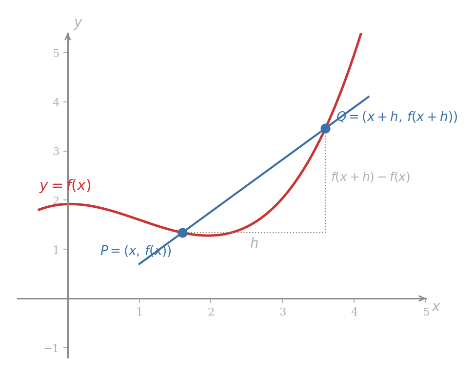
A smooth curve y = f(x) drawn in the plane with two marked points P and Q on it. P is at x-coordinate x with y-coordinate f of x, and Q is at x-coordinate x plus h with y-coordinate f of x plus h. A straight secant line is drawn through P and Q, extending past both. A horizontal dotted segment of length h connects the foot of P with the foot of Q, and a vertical dotted segment of length f of x plus h minus f of x rises from the foot of Q to Q itself, forming the rise-and-run triangle for the secant slope.

The slope of the secant through $P$ and $Q$ is determined by the two points alone, and slope property 2 of Lesson 2AM supplies it directly. Writing $P = (x, f(x))$ and $Q = (x + h,\, f(x + h))$ for some non-zero displacement $h$ , the slope of the secant is

\frac{f(x + h) - f(x)}{(x + h) - x} = \frac{f(x + h) - f(x)}{h},

the difference quotient. The secant line is the geometric object whose slope this quotient computes.

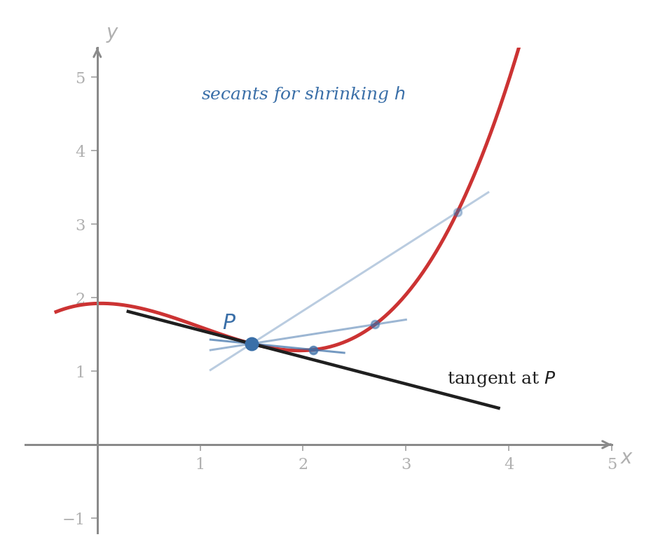
From secant to tangent

Hold $P$ fixed and slide $Q$ along the curve towards $P$ , so that $h$ shrinks towards zero. The secant pivots about $P$ , and if the curve has a tangent line at $P$ the secant approaches that tangent in the same magnification sense as in Lesson 2AM: at progressively smaller $h$ the secant and the tangent become indistinguishable. Translated into numbers, the slope of the secant approaches the slope of the tangent, which is by definition $f'(x)$ .

The same curve y = f(x) with the point P fixed and three secant lines drawn through P and successively closer second points on the curve, each lighter in shade than the last to suggest progression. The actual tangent line at P is drawn as a darker, thicker line, and the secants visibly converge towards the tangent as the second point approaches P.

We record the relationship in standard limit notation,

f'(x) = \lim_{h \to 0} \frac{f(x + h) - f(x)}{h},

the symbol $\lim_{h \to 0}$ being read “the limit as $h$ approaches $0$ of”. The notion of an expression approaching a value will be made more precise in the next section; for now the secant picture is the working intuition.

The substitution $h = 0$ is forbidden in the difference quotient because both numerator and denominator then vanish, leaving the meaningless $0/0$ . The limit allows us nevertheless to read off the value the quotient settles on as $h$ tends to $0$ , without ever setting $h = 0$ .

Three-step recipe

The recipe converts a problem about tangent lines into a problem of algebraic simplification.

Note (Computing $f'(x)$ from the difference quotient)

Write the difference quotient $\dfrac{f(x + h) - f(x)}{h}$ for $h \neq 0$ .
Simplify until the apparent $0/0$ has been removed by algebraic cancellation.
Read off the value the simplified expression approaches as $h \to 0$ . That value is $f'(x)$ .

The first three special cases of the power rule, together with formulas (1) and (2) of the previous section, fall out at once.

Verifying the special cases

Proof

Constant case. Let $f(x) = b$ for some fixed real number $b$ . Then $f(x + h) = b$ for every $h$ , so for every $h \neq 0$ ,

\frac{f(x + h) - f(x)}{h} = \frac{b - b}{h} = \frac{0}{h} = 0.

The constant $0$ approaches $0$ as $h \to 0$ , hence $f'(x) = 0$ .

■

Proof

Linear case. Let $f(x) = mx + b$ . Then

f(x + h) - f(x) = \bigl(m(x + h) + b\bigr) - \bigl(mx + b\bigr) = m h,

and the difference quotient simplifies to $mh / h = m$ for every $h \neq 0$ , the cancellation being legitimate since $h \neq 0$ . The constant $m$ approaches $m$ as $h \to 0$ , so $f'(x) = m$ .

■

Proof

The case $f(x) = x^2$ . Expanding $(x + h)^2 = x^2 + 2 x h + h^2$ ,

\frac{f(x + h) - f(x)}{h} = \frac{(x + h)^2 - x^2}{h} = \frac{2 x h + h^2}{h} = 2x + h

for every $h \neq 0$ . As $h \to 0$ the expression $2x + h$ approaches $2x$ , so $f'(x) = 2x$ , which is the slope formula stated as a Theorem in Lesson 2AM and recovered as formula (3) above.

■

Proof

The case $f(x) = x^3$ . Expanding $(x + h)^3 = x^3 + 3 x^2 h + 3 x h^2 + h^3$ ,

\frac{f(x + h) - f(x)}{h} = \frac{3 x^2 h + 3 x h^2 + h^3}{h} = 3 x^2 + 3 x h + h^2

for every $h \neq 0$ . As $h \to 0$ both terms involving $h$ vanish, so $f'(x) = 3 x^2$ .

■

Example 61 (The case

f(x) = 1/x

)

For $f(x) = 1/x$ on $x \neq 0$ , the difference quotient is

\frac{f(x + h) - f(x)}{h} = \frac{1}{h}\!\left(\frac{1}{x + h} - \frac{1}{x}\right).

Combining the inner fractions over the common denominator $x(x + h)$ ,

\frac{1}{x + h} - \frac{1}{x} = \frac{x - (x + h)}{x(x + h)} = \frac{-h}{x(x + h)},

and substituting back,

\frac{f(x + h) - f(x)}{h} = \frac{-h}{x(x + h) \cdot h} = \frac{-1}{x(x + h)}

for every $h \neq 0$ with $x + h \neq 0$ , the cancellation of $h$ relying on $h \neq 0$ . As $h \to 0$ the denominator approaches $x \cdot x = x^2$ , and the difference quotient approaches $-1/x^2$ . Hence $f'(x) = -1/x^2$ for $x \neq 0$ , in agreement with the power rule at $r = -1$ .

Problem 40

Apply the three-step recipe to compute the derivative of each function below. Indicate at each step where the cancellation $h \neq 0$ is used.

$f(x) = 4 x^2 - 3$ .
$f(x) = x^2 + 2 x + 1$ .
$f(x) = 1/(x + 1)$ on $x \neq -1$ .

Remark

The derivations above prove the power rule for $r = 0, 1, 2, 3$ and for $r = -1$ directly from the limit. The same secant argument with the binomial expansion of $(x + h)^n$ handles every positive integer exponent at once, and slightly more elaborate manipulations recover the rule for negative integers and for rational $r$ . The general statement, together with a more careful theory of limits to back the informal “approaches” used here, awaits a later MA0A lesson.

Limits

The previous section used the phrase “approaches as $h \to 0$ ” without committing to a definition. This section gives a working definition, lists the algebraic rules limits obey, and demonstrates the standard computational tricks for cases where direct substitution fails. A fully formal treatment is left to a later MA0A lesson; for the present we are after enough machinery to compute.

Definition

Definition 24 (Limit of a Function at a Point)

Let $g$ be a function defined on some interval containing the real number $a$ , except possibly at $a$ itself. The number $L$ is the limit of $g(x)$ as $x$ approaches $a$ if $g(x)$ can be made arbitrarily close to $L$ by taking $x$ sufficiently close, but not equal, to $a$ . We write

\lim_{x \to a} g(x) = L.

If no such number $L$ exists, the limit is said to not exist.

The definition examines only the values of $g$ at inputs near $a$ , never at $a$ itself, so $g$ need not be defined at $a$ for the limit to exist. When $g$ is defined at $a$ , the value $g(a)$ may or may not equal the limit; the equality of the two is precisely the property of being continuous at $a$ , taken up below.

Example 62 (Changing the value at the point)

Define

g(x) = \begin{cases} x + 1, & x \neq 2,\\ 100, & x = 2. \end{cases}

For inputs near $2$ but not equal to $2$ , the rule governing $g(x)$ is simply $x + 1$ . Those nearby values approach $3$ as $x$ approaches $2$ , so

\lim_{x \to 2} g(x) = 3.

This does not contradict $g(2) = 100$ : the limit ignores the value at the point itself and reads only the behaviour around it.

Computing a limit from a table

Example 63 (A linear limit by tabulation)

Compute $\displaystyle \lim_{x \to 2}\,(3x - 5)$ .

Tabulating $3x - 5$ at inputs progressively closer to $2$ from each side,

$x$	$3x - 5$	$x$	$3x - 5$
$2.1$	$1.3$	$1.9$	$0.7$
$2.01$	$1.03$	$1.99$	$0.97$
$2.001$	$1.003$	$1.999$	$0.997$
$2.0001$	$1.0003$	$1.9999$	$0.9997$

the outputs from both sides plainly approach $1$ , and they can be made as close to $1$ as desired by taking $x$ close enough to $2$ . Hence $\lim_{x \to 2}\,(3x - 5) = 1$ .

Computing a limit from a graph

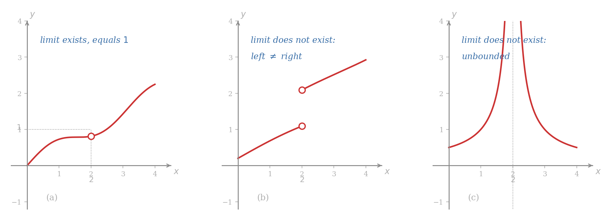
Three side-by-side graphs of functions near x = 2. Panel (a): a smooth curve passes through the level y = 1 at x = 2 with an unfilled circle indicating the function is not defined there; the curve approaches height 1 from both sides. Panel (b): a curve approaches the level 1 as x approaches 2 from the left and approaches the level 2 as x approaches 2 from the right, with unfilled circles at both (2, 1) and (2, 2). Panel (c): two branches of a curve grow without bound on either side of a vertical dotted line at x = 2.

The three panels illustrate the three behaviours that decide whether $\lim_{x \to 2} g(x)$ exists.

In panel (a) the values approach the single number $1$ from both sides, even though $g$ is not defined at $x = 2$ , so the limit exists and equals $1$ . In panel (b) the values approach $1$ from the left and $2$ from the right; the two approaches disagree, so no single number $L$ satisfies the definition and the limit does not exist. In panel (c) the values grow without bound as $x$ approaches $2$ from either side; no real number is approached, and again the limit does not exist.

Limit theorems

The arithmetic operations on functions interact with limits in the most natural way. We list the rules now, deferring the detailed verifications to the later MA0A lesson where the fully formal definition is in place.

Theorem 5 (Limit Theorems)

Suppose $\displaystyle \lim_{x \to a} f(x) = F$ and $\displaystyle \lim_{x \to a} g(x) = G$ both exist. Then:

(I) For every constant $k$ , $\displaystyle \lim_{x \to a} \bigl(k\,f(x)\bigr) = k\,F$ .

(II) For every positive rational $r$ such that $F^r$ is defined and $f(x)^{r}$ is defined on inputs near $a$ other than $a$ itself, $\displaystyle \lim_{x \to a} f(x)^{r} = F^{r}$ .

(III) $\displaystyle \lim_{x \to a} \bigl(f(x) + g(x)\bigr) = F + G$ .

(IV) $\displaystyle \lim_{x \to a} \bigl(f(x) - g(x)\bigr) = F - G$ .

(V) $\displaystyle \lim_{x \to a} \bigl(f(x)\,g(x)\bigr) = F\,G$ .

(VI) If $G \neq 0$ , $\displaystyle \lim_{x \to a} \frac{f(x)}{g(x)} = \frac{F}{G}$ .

The two further consequences below are the most often invoked and are derived from the rules above without further input.

Theorem 6 (Limits of Polynomial and Rational Functions)

Let $a$ be a real number.

(VII) For every polynomial function $p$ , $\displaystyle \lim_{x \to a} p(x) = p(a)$ .

(VIII) For every rational function $r = p/q$ with $q(a) \neq 0$ , $\displaystyle \lim_{x \to a} r(x) = r(a)$ .

In short: for polynomial and rational functions, the limit at any point of the natural domain is found by direct substitution.

Proof

(VII) The constant function with value $c$ has $\lim_{x \to a} c = c$ , since the constant value $c$ is already arbitrarily close to itself for every input. The identity function has $\lim_{x \to a} x = a$ by inspection, since taking $x$ close to $a$ makes $x$ itself close to $a$ . Limit Theorem II applied to the identity gives $\lim_{x \to a} x^{n} = a^{n}$ for every positive integer $n$ , since the integer power is the rational power $r = n$ . Limit Theorem I then gives $\lim_{x \to a} c_{n}\,x^{n} = c_{n}\,a^{n}$ for each coefficient, and Limit Theorem III applied across the finite sum that defines $p$ recombines these into $p(a)$ .

(VIII) With $\lim_{x \to a} p(x) = p(a)$ and $\lim_{x \to a} q(x) = q(a) \neq 0$ , Limit Theorem VI gives $\lim_{x \to a} (p(x)/q(x)) = p(a)/q(a) = r(a)$ .

■

Worked computations

Example 64 (Direct substitution suffices)

By Theorem VII applied to the polynomial $5 x^{3} - 15$ ,

\lim_{x \to 2} \bigl(5 x^{3} - 15\bigr) = 5 \cdot 2^{3} - 15 = 25.

Limit Theorem II with $r = \tfrac{1}{2}$ then gives

\lim_{x \to 2} \sqrt{5 x^{3} - 15} = 25^{1/2} = 5,

and Limit Theorem VI with the polynomial $x^{5}$ in the denominator (non-zero at $x = 2$ ) supplies

\lim_{x \to 2} \frac{\sqrt{5 x^{3} - 15}}{x^{5}} = \frac{5}{32}.

When direct substitution returns the indeterminate form $0/0$ , no theorem applies until algebra has cleared the obstruction. Two algebraic moves cover almost every elementary case: factoring, and rationalising.

Example 65 (Factoring out the obstruction)

Compute $\displaystyle \lim_{x \to 3} \frac{x^{2} - 9}{x - 3}$ .

Direct substitution gives $\tfrac{0}{0}$ . Factoring the numerator,

\frac{x^{2} - 9}{x - 3} = \frac{(x - 3)(x + 3)}{x - 3} = x + 3 \qquad (x \neq 3),

the cancellation legitimate because the limit examines only $x \neq 3$ . The right-hand side is a polynomial, so by Theorem VII its limit at $3$ is $3 + 3 = 6$ , and so the original limit equals $6$ .

Remark (Same expression, different functions)

The two formulas

f(x) = \frac{x^{2} - 9}{x - 3} \qquad \text{and} \qquad g(x) = x + 3

agree at every $x \neq 3$ , but they are not the same function. The natural domain of $f$ excludes $x = 3$ , where the denominator vanishes; the domain of $g$ is the whole real line. The graph of $f$ therefore matches that of $g$ everywhere except for a single missing point at $(3, 6)$ .

Because the limit ignores the value at $x = 3$ entirely, the two functions have the same limit there: $\lim_{x \to 3} f(x) = \lim_{x \to 3} g(x) = 6$ . Direct substitution succeeds for $g$ but fails for $f$ , even though the answer it would yield, were it permitted, is correct. The cancellation step in the example above is the formal acknowledgement that the limit cares only about the agreement of $f$ and $g$ on the inputs near but not equal to $3$ .

Example 66 (Rationalising the obstruction)

Compute $\displaystyle \lim_{x \to 0} \frac{\sqrt{x + 4} - 2}{x}$ .

Direct substitution again gives $\tfrac{0}{0}$ . Multiplying numerator and denominator by the conjugate $\sqrt{x + 4} + 2$ ,

\frac{\sqrt{x + 4} - 2}{x} \cdot \frac{\sqrt{x + 4} + 2}{\sqrt{x + 4} + 2} = \frac{(x + 4) - 4}{x \bigl(\sqrt{x + 4} + 2\bigr)} = \frac{1}{\sqrt{x + 4} + 2}

for every $x \neq 0$ , the cancellation again legitimate because the limit excludes $x = 0$ . The denominator is now a sum of a square root and a constant, both well-behaved at $x = 0$ , and Limit Theorem VI together with Theorem II gives

\lim_{x \to 0} \frac{\sqrt{x + 4} - 2}{x} = \frac{1}{\sqrt{0 + 4} + 2} = \frac{1}{4}.

Problem 41

Compute each limit, citing the theorem or algebraic step used at each line.

$\displaystyle \lim_{x \to -1} \bigl(x^{4} - 3 x^{2} + 2 x\bigr)$ .
$\displaystyle \lim_{x \to 4} \frac{x^{2} - 16}{x - 4}$ .
$\displaystyle \lim_{x \to 0} \frac{\sqrt{1 + x} - 1}{x}$ .
$\displaystyle \lim_{x \to 2} \frac{x^{3} - 8}{x - 2}$ .

Remark

The cancellation step in each algebraic move rests on the fact that the limit ignores the value of the function at the point itself, examining only the surrounding inputs. The same move was at the heart of the difference-quotient calculations of the previous section: cancelling $h$ in $(f(x + h) - f(x))/h$ was legitimate precisely because $h \neq 0$ throughout the limit. Limits and the difference-quotient computations are therefore the same algebraic procedure dressed in different geometric clothing.

The Limit Definition of the Derivative

The two previous sections together supply the missing ingredient. The limit is now defined, and the informal “approaches” used in the secant construction admit a precise reading. The derivative therefore admits a definition that no longer relies on the geometric picture of the tangent line; the picture is recovered as a consequence whenever the curve has a tangent at the point in question.

Definition 25 (Derivative as a Limit)

A function $f$ is differentiable at the input $x$ if the difference quotient

\frac{f(x + h) - f(x)}{h}

has a limit as $h$ approaches $0$ . When this limit exists, its value is the derivative of $f$ at $x$ , written

f'(x) = \lim_{h \to 0} \frac{f(x + h) - f(x)}{h}.

If the limit does not exist, $f$ is nondifferentiable at $x$ .

The geometric reading of $f'(x)$ as the slope of the tangent line is recovered whenever the curve $y = f(x)$ has a tangent at $(x, f(x))$ , since the secant slopes then approach the tangent slope as $h \to 0$ . Most functions in the early part of this course are differentiable at most inputs of their natural domains; exceptions include corners such as $|x|$ at $0$ , vertical tangents such as $\sqrt{x}$ at $0$ , and points excluded from the natural domain in the first place. These exceptions are catalogued below and treated more systematically in later MA0A lessons.

The three-step recipe in limit notation

The recipe of the previous section restates without change, now backed by the limit definition.

Note (Computing $f'(x)$ from the definition)

Write the difference quotient $\dfrac{f(x + h) - f(x)}{h}$ for $h \neq 0$ .
Simplify algebraically until the cancellation $h \neq 0$ has done its work.
Take the limit as $h \to 0$ , using limit theorems VII and VIII where applicable. The value is $f'(x)$ .

The recipe produces either a number or a function depending on what is asked: holding $x = a$ throughout produces the derivative at $a$ , the single number $f'(a)$ ; carrying $x$ symbolically produces the derivative function $f'$ , whose value at any chosen input can then be read off. The two outputs are distinct objects and should be kept apart.

Computing $f'(a)$ at a specific input

Example 67 (

f(x) = 15 - x^2

a = 5

)

Step 1. With $f(5) = 15 - 25 = -10$ and $f(5 + h) = 15 - (5 + h)^2$ ,

\frac{f(5 + h) - f(5)}{h} = \frac{15 - (25 + 10 h + h^2) - (-10)}{h} = \frac{-10 h - h^2}{h}.

Step 2. Cancelling $h \neq 0$ ,

\frac{-10 h - h^2}{h} = -10 - h.

Step 3. By Limit Theorem VII applied to the polynomial $-10 - h$ ,

f'(5) = \lim_{h \to 0} (-10 - h) = -10.

Example 68 (

f(x) = 1/(2 x - 3)

a = 5

)

Step 1. With $f(5) = 1/7$ and $f(5 + h) = 1/(2(5 + h) - 3) = 1/(7 + 2 h)$ ,

\frac{f(5 + h) - f(5)}{h} = \frac{1}{h}\!\left(\frac{1}{7 + 2 h} - \frac{1}{7}\right).

Step 2. Combining the inner fractions over the common denominator $7\,(7 + 2 h)$ ,

\frac{1}{7 + 2 h} - \frac{1}{7} = \frac{7 - (7 + 2 h)}{7\,(7 + 2 h)} = \frac{-2 h}{7\,(7 + 2 h)},

so the difference quotient simplifies to

\frac{-2 h}{h \cdot 7\,(7 + 2 h)} = \frac{-2}{49 + 14 h},

the cancellation of $h$ legitimate because $h \neq 0$ .

Step 3. By Limit Theorem VIII applied to the rational function $-2/(49 + 14 h)$ ,

f'(5) = \lim_{h \to 0} \frac{-2}{49 + 14 h} = -\frac{2}{49}.

Example 69 (Instantaneous speed of a moving body)

A car begins to move at time $t = 0$ , and its distance from the start in feet after $t$ seconds is recorded as $d(t) = 3 t^{2} - t$ . The average speed over any interval from $t = 1$ to $t = 1 + h$ seconds is the distance covered divided by the elapsed time,

\frac{d(1 + h) - d(1)}{(1 + h) - 1} = \frac{d(1 + h) - d(1)}{h},

the same difference quotient that defines $d'(1)$ . The instantaneous speed of the car at $t = 1$ is the limit of these average speeds as the interval shrinks, that is, $d'(1)$ .

Tabulating the average speeds for shrinking $h$ gives a numerical sense of the limit:

$h$	average speed (ft/s)
$1$	$8$
$0.1$	$5.3$
$0.01$	$5.03$
$0.001$	$5.003$

The values plainly approach $5$ . To confirm by direct computation, expand

d(1 + h) - d(1) = 3(1 + h)^{2} - (1 + h) - (3 - 1) = (3 + 6 h + 3 h^{2}) - 1 - h - 2 = 5 h + 3 h^{2},

so the average speed is $5 + 3 h$ for $h \neq 0$ . By Limit Theorem VII applied to the polynomial $5 + 3 h$ in $h$ ,

d'(1) = \lim_{h \to 0}(5 + 3 h) = 5

feet per second. The reading of $d'(1)$ as instantaneous speed is the temporal counterpart of the slope-of-tangent reading: an average rate over an interval is sent to its limit as the interval shrinks, and the result is the rate at the single instant.

Computing a derivative formula

Example 70 (

f(x) = x^2 + 2 x + 2

)

Step 1. Expanding $f(x + h) = (x + h)^2 + 2(x + h) + 2 = x^2 + 2 x h + h^2 + 2 x + 2 h + 2$ and subtracting $f(x) = x^2 + 2 x + 2$ ,

f(x + h) - f(x) = 2 x h + h^2 + 2 h.

Step 2. Dividing by $h$ and cancelling,

\frac{f(x + h) - f(x)}{h} = 2 x + h + 2.

Step 3. By Limit Theorem VII applied to the polynomial $2 x + h + 2$ in the variable $h$ ,

f'(x) = \lim_{h \to 0} (2 x + h + 2) = 2 x + 2.

The output is a function; evaluating it at any specific input gives the corresponding derivative value, for example $f'(0) = 2$ , $f'(1) = 4$ , $f'(-1) = 0$ .

Verifying the Power Rule from the limit

The power rule was stated without proof and verified by hand for $r = 0, 1, 2, 3$ in the secant section, and the case $r = -1$ was treated alongside as $f(x) = 1/x$ . The case $r = \tfrac{1}{2}$ is the next standard one, predicted by the rule to yield $f'(x) = \tfrac{1}{2}\,x^{-1/2} = 1/(2 \sqrt{x})$ .

Proof

The case $f(x) = \sqrt{x}$ on $x > 0$ . Rationalising the difference quotient by multiplying numerator and denominator by the conjugate $\sqrt{x + h} + \sqrt{x}$ ,

\frac{\sqrt{x + h} - \sqrt{x}}{h} \cdot \frac{\sqrt{x + h} + \sqrt{x}}{\sqrt{x + h} + \sqrt{x}} = \frac{(x + h) - x}{h\,\bigl(\sqrt{x + h} + \sqrt{x}\bigr)} = \frac{1}{\sqrt{x + h} + \sqrt{x}}

for every $h \neq 0$ with $x + h > 0$ , the cancellation of $h$ legitimate because $h \neq 0$ . As $h \to 0$ the denominator approaches $\sqrt{x} + \sqrt{x} = 2 \sqrt{x}$ by limit theorems II and III applied to the square-root expression, so

f'(x) = \lim_{h \to 0} \frac{1}{\sqrt{x + h} + \sqrt{x}} = \frac{1}{2 \sqrt{x}},

in agreement with the power rule at $r = \tfrac{1}{2}$ .

■

Recognising a limit as a derivative

The defining formula reads in both directions. A limit of the form $\lim_{h \to 0} (f(a + h) - f(a))/h$ is by definition $f'(a)$ , so a limit that can be massaged into this shape computes a derivative at a point and yields its value via the power rule or any other available calculation.

Example 71 (A cube-root limit)

Compute $\displaystyle \lim_{x \to 0} \frac{(1 + x)^{1/3} - 1}{x}$ .

Renaming the dummy variable $x$ as $h$ leaves the limit unchanged,

\lim_{x \to 0} \frac{(1 + x)^{1/3} - 1}{x} = \lim_{h \to 0} \frac{(1 + h)^{1/3} - 1}{h}.

Setting $f(x) = x^{1/3}$ and $a = 1$ , the right-hand side is exactly $f'(1)$ by the limit definition. The power rule with $r = \tfrac{1}{3}$ gives $f'(x) = \tfrac{1}{3}\,x^{-2/3}$ , so

f'(1) = \tfrac{1}{3} \cdot 1^{-2/3} = \tfrac{1}{3},

and therefore the original limit equals $\tfrac{1}{3}$ .

Problem 42

Apply the limit definition step by step.

Compute $f'(3)$ for $f(x) = 2 x^2 + x - 1$ .
Find the derivative formula of $f(x) = 1/(x + 3)$ on $x \neq -3$ , then evaluate at $a = 1$ .

Problem 43

Recognise each limit as $f'(a)$ for a suitable $f$ and $a$ , and evaluate it via the power rule.

$\displaystyle \lim_{h \to 0} \frac{(2 + h)^4 - 16}{h}$ .
$\displaystyle \lim_{h \to 0} \frac{\sqrt{9 + h} - 3}{h}$ .
$\displaystyle \lim_{h \to 0} \frac{1/(4 + h) - 1/4}{h}$ .

Limits at Infinity

The limits considered so far have all sent $x$ towards a fixed real number $a$ . A second style of limit asks what the function does as $x$ grows without bound, in either the positive or the negative direction. The behaviour at infinity is what records, for instance, that a graph approaches a fixed horizontal line, called a horizontal asymptote, or that a quantity stabilises in the long run.

Definition 26 (Limit at Infinity)

Let $g$ be a function defined on every input larger than some threshold. The number $L$ is the limit of $g(x)$ as $x$ approaches $\infty$ if $g(x)$ can be made arbitrarily close to $L$ by taking $x$ sufficiently large; we then write

\lim_{x \to \infty} g(x) = L.

The corresponding statement with “sufficiently large” replaced by “sufficiently large in magnitude with $x$ negative” defines $\lim_{x \to -\infty} g(x) = L$ .

The symbol $\infty$ is not a real number; the notation $x \to \infty$ describes a direction in which $x$ is sent to grow, not a value at which it arrives.

Two side-by-side panels. The left panel shows a curve that rises from below toward the horizontal dashed line y = 2, getting closer to it as x grows large to the right; the panel is labelled limit as x approaches infinity equals 2. The right panel shows a curve that approaches the horizontal dashed line y = 0 from above as x grows large in the negative direction; the panel is labelled limit as x approaches minus infinity equals 0.

The arithmetic limit theorems of the previous section apply to limits at infinity in the examples below. The polynomial-and-rational direct-substitution rule (Theorem VIII) is replaced, for rational functions, by the algebraic divide-by-the-largest-power trick illustrated below.

Computing limits at infinity

Example 72 (Two limits at

\infty

)

Part (a). Compute $\displaystyle \lim_{x \to \infty} \frac{1}{x^{2} + 1}$ .

As $x$ grows large the polynomial $x^{2} + 1$ grows without bound, so its reciprocal $1/(x^{2} + 1)$ becomes arbitrarily small in magnitude. The limit is therefore $0$ .

Part (b). Compute $\displaystyle \lim_{x \to \infty} \frac{6 x - 1}{2 x + 1}$ .

Both numerator and denominator grow without bound, so direct inspection is inconclusive. Dividing numerator and denominator by $x$ (legitimate since $x > 0$ once $x$ is large),

\frac{6 x - 1}{2 x + 1} = \frac{6 - 1/x}{2 + 1/x}.

As $x \to \infty$ , the term $1/x$ approaches $0$ , so by limit theorems III and IV the numerator approaches $6$ and the denominator approaches $2$ , and Limit Theorem VI then gives

\lim_{x \to \infty} \frac{6 x - 1}{2 x + 1} = \frac{6}{2} = 3.

Problem 44

Compute each of the following limits.

$\displaystyle \lim_{x \to \infty} \frac{1}{x^{2}}$ .
$\displaystyle \lim_{x \to -\infty} \frac{1}{x^{2}}$ .
$\displaystyle \lim_{x \to \infty} \frac{5 x + 3}{3 x - 2}$ .
$\displaystyle \lim_{x \to \infty} \frac{1}{x - 8}$ .

Limit theorems applied at infinity

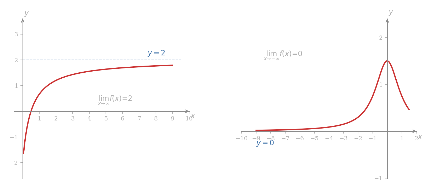
The arithmetic rules (I)–(VI) of the previous section read identically for limits at infinity, and the same algebra recombines limits of constituent expressions into the limit of a combination. The next example applies the rules to information read off a graph.

Example 73 (Combining a graphed limit with the rules)

Suppose a function $f$ satisfies $\displaystyle \lim_{x \to \infty} f(x) = 2$ , as one might read off a horizontal asymptote drawn into a graph. By limit theorems IV and I,

\lim_{x \to \infty} \bigl(1 - 3 f(x)\bigr) = \lim_{x \to \infty} 1 - 3 \lim_{x \to \infty} f(x) = 1 - 3 \cdot 2 = -5,

the constant $1$ contributing its own value $1$ as a constant limit. By Limit Theorem II with $r = 2$ ,

\lim_{x \to \infty} f(x)^{2} = \Bigl(\lim_{x \to \infty} f(x)\Bigr)^{2} = 2^{2} = 4.

Both calculations rest only on the value $\lim_{x \to \infty} f(x) = 2$ ; no further information about $f$ is needed.

Reading limits from a graph

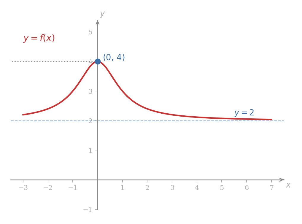
A smooth curve y = f(x) drawn over the interval from x = -3 to x = 7. The curve passes through the marked point (0, 4) at the y-axis, descends symmetrically to either side toward the horizontal dashed asymptote y = 2 that the curve approaches as x grows large in either direction. Dotted reference lines are drawn from (0, 4) to both axes.

The function $f$ graphed above satisfies $\lim_{x \to 0} f(x) = 4$ (the value $f(0) = 4$ being attained continuously) and $\lim_{x \to \infty} f(x) = 2$ (the horizontal asymptote $y = 2$ ). Each of the limits below combines these two facts through the limit theorems of the previous section.

Problem 45

Refer to the graph above for the values of $f$ . Compute each limit.

$\displaystyle \lim_{x \to 0} f(x)$ .
$\displaystyle \lim_{x \to \infty} f(x)$ .
$\displaystyle \lim_{x \to 0} x\,f(x)$ .
$\displaystyle \lim_{x \to \infty} \bigl(1 + 2 f(x)\bigr)$ .
$\displaystyle \lim_{x \to \infty} \bigl(1 - f(x)\bigr)$ .
$\displaystyle \lim_{x \to 0} f(x)^{2}$ .

Remark

The two limit styles, $x \to a$ and $x \to \pm\infty$ , share the same algebraic intuition: the value the function settles on as the input is sent to a chosen limiting position. The mechanical difference is that $\infty$ is not a real number and cannot be substituted into a formula. For rational functions, direct evaluation is replaced by the divide-by-the-largest-power trick of the worked example. The two styles together cover almost every limit needed in the lessons ahead.

Differentiability and Continuity

The limit definition of the derivative declared $f$ to be differentiable at $x$ when the difference-quotient limit exists, and nondifferentiable otherwise. Up to now this exception has been a footnote: most of the functions in the course are differentiable at every input of their natural domain. The exceptions arise in applied problems (a tariff that changes its rate at a threshold produces one) and sit at the boundary between continuity and the stronger notion of differentiability. This section catalogues the failure modes for each, shows that differentiability is the stricter condition, and gives the standard continuity statements for polynomial and rational functions.

Geometric failures of differentiability

A function fails to be differentiable at an input $a$ in one of three principal ways, each visible in the shape of the graph at $(a, f(a))$ .

Three side-by-side panels each showing a curve with a marked point at x = a. The left panel shows a V-shaped graph meeting at a sharp corner over a, labelled 'corner: no tangent'. The middle panel shows a smooth curve through a with the curve's tangent direction at a being vertical, labelled 'vertical tangent at a'. The right panel shows a curve in two pieces with a visible vertical jump at x = a, labelled 'jump: graph broken at a'.

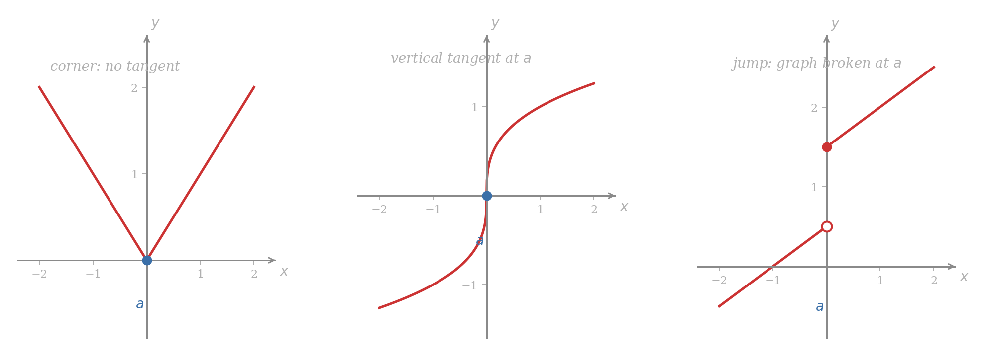
The three failure modes admit clean descriptions in the language already in place.

A corner at $a$ , like the absolute value graph $y = |x|$ at the origin from Lesson 1PM, has the property that the secant slopes computed from the right approach a different value from the secant slopes computed from the left. The difference-quotient limit therefore fails to exist and $f'(a)$ is undefined.

A vertical tangent at $a$ , like the cube root $y = x^{1/3}$ at the origin, has the property that the secant slopes grow without bound as $h$ approaches $0$ . No real number is approached, so once again the limit fails and $f'(a)$ is undefined; geometrically, slope is not defined for vertical lines.

A jump at $a$ leaves the function discontinuous there, and a discontinuity prevents differentiability outright by the theorem of the next subsection.

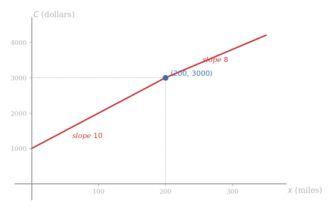
A piecewise tariff with a corner

Example 74 (A railway haulage charge)

A goods rail operator quotes a flat handling fee of $\pounds 1{,}000$ per wagon, plus $\pounds 10$ per mile for the first $200$ miles and $\pounds 8$ for each additional mile past $200$ . Writing $C(x)$ for the total charge of sending a wagon $x$ miles,

C(x) = \begin{cases} 1000 + 10\,x, & 0 \leq x \leq 200, \\ 1400 + 8\,x, & x > 200, \end{cases}

where the second clause comes from $C(200) + 8(x - 200) = 3000 + 8x - 1600 = 1400 + 8x$ . The two pieces agree in value at the boundary $x = 200$ , both giving $C(200) = 3000$ , so the graph has no jump.

The slopes of the two pieces are different: $10$ on the left, $8$ on the right. The graph therefore has a corner at $x = 200$ , and $C$ is non-differentiable there even though it is continuous. Every tariff that switches its per-unit rate at a threshold has the same shape.

The graph of the cost function C(x) for railway haulage. The graph is two straight-line segments joined at the marked point (200, 3000): the left segment has slope 10 and runs from (0, 1000) to (200, 3000), and the right segment has slope 8 and continues from (200, 3000) onwards with a noticeably gentler rise. Dotted reference lines drop from (200, 3000) to both axes.

Problem 46

A delivery van charges $\pounds 5$ per kilometre for the first kilometre and $\pounds 2$ per kilometre after that, with no fixed fee. Write the cost $C(x)$ of an $x$ -kilometre delivery as a piecewise function, sketch the graph, identify the input at which $C$ is non-differentiable, and explain why the two slopes are not equal there.

Continuity informally

Differentiability turned on the existence of a limit; continuity turns on a softer condition that the graph have no breaks. Informally, $f$ is continuous at $a$ when the graph passes through $(a, f(a))$ without lifting the pen from the paper. Many functions whose graphs have appeared so far are continuous on their natural domains even when they fail to be differentiable: the absolute value function is continuous at its corner, and the piecewise tariff above is continuous at its boundary despite the change in slope.

A discontinuity is more violent: the function value at $a$ either fails to exist or sits in a different place from the values nearby. The next example is honest about how this can happen in practice.

A piecewise schedule with jumps

Example 75 (A factory cost with shift overheads)

A plant produces up to $15{,}000$ units in one $8$ -hour shift. Each shift carries a fixed overhead of $\pounds 2{,}000$ for power, supervision, and the like, and the variable cost of materials and direct labour is $\pounds 2$ per unit. Writing $C(x)$ for the cost of producing $x$ units in a single day,

C(x) = \begin{cases} 2{,}000 + 2 x, & 0 \leq x \leq 15{,}000, \\ 4{,}000 + 2 x, & 15{,}000 < x \leq 30{,}000, \\ 6{,}000 + 2 x, & 30{,}000 < x \leq 45{,}000. \end{cases}

Each new shift adds another $\pounds 2{,}000$ to the fixed overhead. At the boundary $x = 15{,}000$ the first formula gives $32{,}000$ while the second formula gives $34{,}000$ at any value just above $15{,}000$ ; the jump of $\pounds 2{,}000$ is the cost of opening a second shift. A second jump of the same size occurs at $x = 30{,}000$ when a third shift becomes necessary.

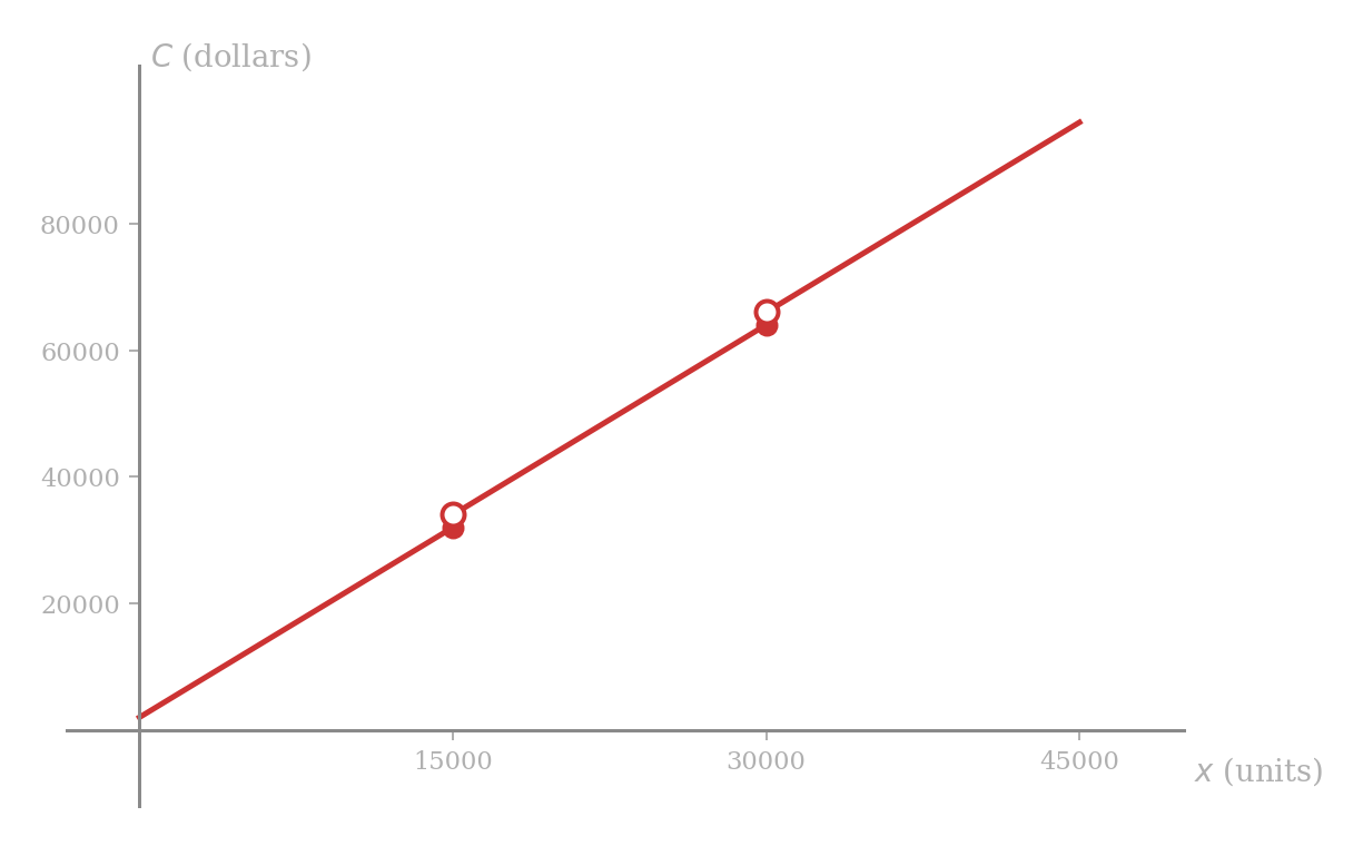
The graph of the manufacturing cost function C(x) over the interval from 0 to 45,000 units. The graph is in three straight segments, each with slope 2: the first runs from (0, 2000) to (15000, 32000), then jumps upward by 2000 to (15000, 34000) where the second segment begins and rises to (30000, 64000), then jumps upward again by 2000 to (30000, 66000) where the third segment begins and rises to (45000, 96000). The endpoints of each segment at the jump are drawn with filled and unfilled circles indicating which side of the boundary each value belongs to.

The graph has visible breaks at $x = 15{,}000$ and $x = 30{,}000$ . A factory manager facing the second of these breaks can either decline an order that would push production above the threshold or accept the $\pounds 2{,}000$ overhead; the discontinuity is what makes that decision a discrete one rather than a marginal one.

Continuity in limit terms

The informal “no break” reading is captured precisely by the limit construction of the previous sections.

Definition 27 (Continuity at a Point)

A function $f$ is continuous at the point $a$ if

\lim_{x \to a} f(x) = f(a).

The function is continuous on an interval, or on a specified collection of inputs, if it is continuous at every point under consideration.

For the equality above to hold, three separate conditions must be satisfied:

$f(a)$ must be defined; that is, $a$ must lie in the domain of $f$ .
$\lim_{x \to a} f(x)$ must exist.
The limit and the value must agree.

A failure of any single condition produces a failure of continuity at $a$ .

Four side-by-side panels labelled (a) through (d), each showing a curve near x = 3. Panel (a): a continuous curve passes through the level y = 2 at x = 3 (with an unfilled circle), but a separate filled point (3, 4) sits above it, indicating that the limit equals 2 but the value f(3) equals 4. Panel (b): the curve has a jump discontinuity at x = 3, with the left piece ending at one height with a filled circle and the right piece starting at a higher level with an unfilled circle. Panel (c): the curve has two branches that grow without bound on either side of x = 3, with a vertical dotted asymptote drawn at x = 3. Panel (d): the curve is a single continuous-looking arc with an unfilled circle at x = 3 indicating the function is undefined there.

Example 76 (Four ways to fail continuity at

x = 3

)

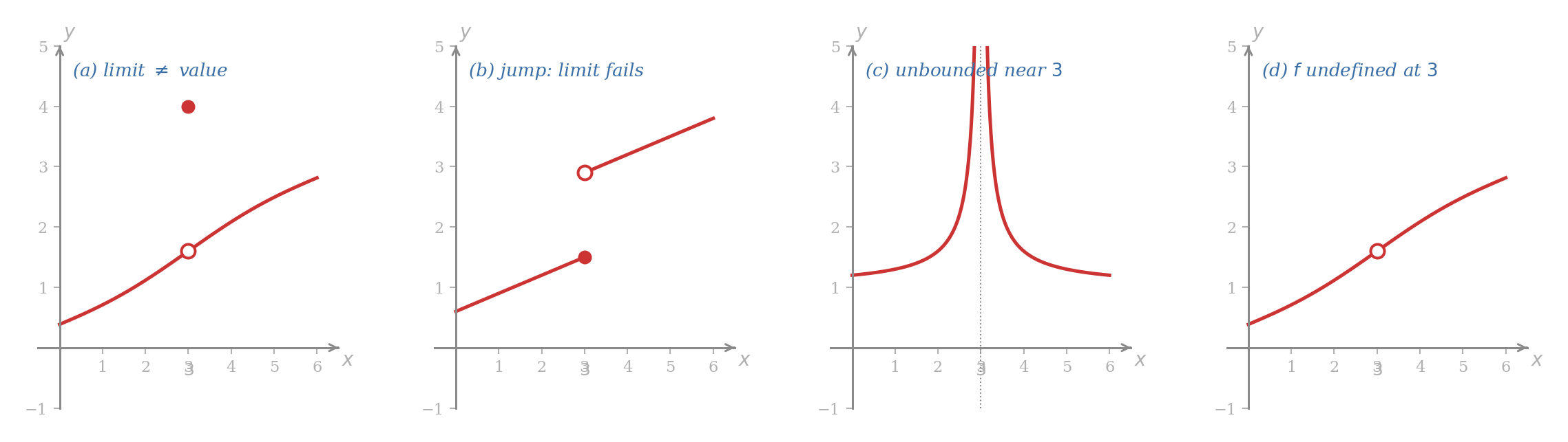
The four panels above each show a function that fails to be continuous at $x = 3$ , illustrating different failure conditions.

Panel (a). $\lim_{x \to 3} f(x) = 2$ exists, and $f(3) = 4$ is defined, but the two disagree. Condition 3 fails.

Panel (b). $\lim_{x \to 3} g(x)$ does not exist, the values approached from the left and right being different. Condition 2 fails.

Panel (c). $\lim_{x \to 3} h(x)$ does not exist, the values growing without bound on either side. Condition 2 fails.

Panel (d). $f(3)$ is not defined; there is no value to compare the limit against. Condition 1 fails.

Problem 47

For each function below, state whether it is continuous at the indicated input, and if not, identify which of the three conditions in the continuity definition fails.

$f(x) = (x^2 - 1)/(x - 1)$ at $x = 1$ .
$g(x) = \begin{cases} x^2, & x < 0, \\ x + 1, & x \geq 0 \end{cases}$ at $x = 0$ .
$h(x) = 1/x$ at $x = 0$ .

Continuity of polynomial and rational functions

The limit theorems of the polynomial and rational sections turn into continuity statements at every input of the natural domain.

Theorem 7 (Continuity of Polynomial and Rational Functions)

Every polynomial function $p$ is continuous at every real number. Every rational function $r = p/q$ is continuous at every real number $a$ with $q(a) \neq 0$ .

Proof

For the polynomial case, Limit Theorem VII of the previous section gives $\lim_{x \to a} p(x) = p(a)$ at every real $a$ . The continuity definition asks for exactly this equality, so $p$ is continuous at every $a$ .

For the rational case, the natural domain of $r = p/q$ excludes precisely those $a$ with $q(a) = 0$ . At every other $a$ , Limit Theorem VIII gives $\lim_{x \to a} r(x) = r(a)$ , and the continuity definition is again satisfied.

■

In particular, every algebraic function written as a polynomial or rational expression is continuous on its natural domain, and the same applies to power functions $x^r$ at every input where the power is defined. The exceptional inputs for which continuity must be checked individually include boundaries between piecewise definitions, roots of denominators, and other inputs where the formula changes its behaviour.

Differentiability is stronger than continuity

The two notions are related, but unequally so.

Theorem 8 (Differentiability Implies Continuity)

If $f$ is differentiable at $a$ , then $f$ is continuous at $a$ .

The converse is false. The absolute value function from Lesson 1PM is continuous at the origin (the two pieces agree in value there) but not differentiable there (the two pieces disagree in slope), and the haulage cost example above is continuous at $x = 200$ but not differentiable there for the same reason. Continuity is the strictly weaker requirement.

Proof

Differentiability implies continuity. Suppose $f$ is differentiable at $a$ , so the limit

f'(a) = \lim_{h \to 0} \frac{f(a + h) - f(a)}{h}

exists as a real number. The continuity condition at $a$ is $\lim_{x \to a} f(x) = f(a)$ , equivalently $\lim_{x \to a}(f(x) - f(a)) = 0$ . Setting $x = a + h$ , with $x \to a$ if and only if $h \to 0$ , the equivalent form becomes $\lim_{h \to 0}(f(a + h) - f(a)) = 0$ .

For $h \neq 0$ we may write

f(a + h) - f(a) = \frac{f(a + h) - f(a)}{h} \cdot h.

By Limit Theorem V applied to the product on the right,

\lim_{h \to 0}\bigl(f(a + h) - f(a)\bigr) = \Bigl(\lim_{h \to 0} \frac{f(a + h) - f(a)}{h}\Bigr) \cdot \Bigl(\lim_{h \to 0} h\Bigr) = f'(a) \cdot 0 = 0,

the first factor existing by the differentiability hypothesis and the second factor being trivially zero. Hence $\lim_{x \to a}(f(x) - f(a)) = 0$ , equivalently $\lim_{x \to a} f(x) = f(a)$ , and $f$ is continuous at $a$ .

■

Equivalently, a function that is not continuous at $a$ cannot be differentiable at $a$ . The manufacturing cost above is therefore non-differentiable at both $x = 15{,}000$ and $x = 30{,}000$ , where it is discontinuous; the railway haulage cost is non-differentiable at $x = 200$ , where it is continuous but cornered.

Remark

The chain of implications and exceptions can be summarised in two sentences: if $f$ is differentiable at $a$ , then $f$ is continuous at $a$ ; if $f$ is continuous at $a$ , it does not necessarily follow that $f$ is differentiable at $a$ .

The direction matters. Honesty about it protects us from the standard error of trying to read $f'(a)$ off a graph that has a jump or a corner there.

Problem 48

For each function below, decide whether $f$ is continuous at $a$ , and whether $f$ is differentiable at $a$ . Use the failure mode (corner, vertical tangent, or discontinuity) where appropriate.

$f(x) = |x - 5|$ at $a = 5$ .
$f(x) = x^{1/3}$ at $a = 0$ .
$f(x) = (x^2 - 4)/(x - 2)$ at $a = 2$ .
$f(x) = \begin{cases} 3 - x, & x < 1, \\ x^2 + 1, & x \geq 1 \end{cases}$ at $a = 1$ .

Video

Lesson assets

Limits and Derivatives

The Derivative

Linear and constant functions

The cases x2x^2x2 and x3x^3x3

The Power Rule

Geometric Meaning and the Tangent Line

Equation of the tangent line at x=ax = ax=a

Operator notation

The Secant Line and the Derivative

Secant lines

From secant to tangent

Three-step recipe

Verifying the special cases

Limits

Definition

Computing a limit from a table

Computing a limit from a graph

Limit theorems

Worked computations

The Limit Definition of the Derivative

The three-step recipe in limit notation

Computing f′(a)f'(a)f′(a) at a specific input

Computing a derivative formula

Verifying the Power Rule from the limit

Recognising a limit as a derivative

Limits at Infinity

Computing limits at infinity

Limit theorems applied at infinity

Reading limits from a graph

Differentiability and Continuity

Geometric failures of differentiability

A piecewise tariff with a corner

Continuity informally

A piecewise schedule with jumps

Continuity in limit terms

Continuity of polynomial and rational functions

Differentiability is stronger than continuity

The cases $x^2$ and $x^3$

Equation of the tangent line at $x = a$

Computing $f'(a)$ at a specific input