16/02/2026

#Math#Differentiation

Video

Lesson assets

video link

CS50P Lecture 0: Functions, Variables

exercise

Exercise 2 PDF

Slopes and Rates of Change

Rates of Change

Lesson 1 isolated the slope of a linear function as the geometric record of how its output responds to its input. For $f(x) = mx + b$ the AM linear function definition fixed $m$ as the number of vertical units gained for each unit step to the right, and the picture made the sign of $m$ visible: rising lines have $m > 0$ , falling lines have $m < 0$ , level lines have $m = 0$ , and the steeper the line the larger $|m|$ is. The same number admits a second reading.

Definition 18 (Rate of Change of a Linear Function)

The rate of change of the linear function $f(x) = mx + b$ is its slope $m$ . Concretely, when the input is increased by any amount $h$ , the output changes by exactly $m h$ , regardless of the input from which the increase begins.

The constancy of this number is the defining feature of linearity: a single value of $m$ describes the response of $f$ at every point of its domain. Choosing any base point $x_0$ and shifting to $x_0 + h$ ,

f(x_0 + h) - f(x_0) = \bigl(m(x_0 + h) + b\bigr) - \bigl(m x_0 + b\bigr) = m h,

which depends on $h$ but not on $x_0$ . Dividing by $h$ recovers $m$ , the slope, on the nose. For this division we assume $h \neq 0$ ; when $h = 0$ the output change is $0$ but the quotient is undefined.

When the linear function carries a physical meaning, its rate of change inherits one too. The PM lesson’s printing-cost example is a typical case: a publisher whose total cost satisfies $C(x) = 10{,}000 + 25 x$ pays a fixed overhead of $\pounds 10{,}000$ at the $y$ -intercept and an additional $\pounds 25$ for each further copy, so the slope $25$ is the cost incurred when one more copy is produced. This unit-step reading of the slope is common enough in cost models to deserve a name of its own.

Definition 19 (Marginal Cost)

For a linear cost function $C(x) = m x + b$ giving the total cost of producing $x$ units of a commodity, the slope $m$ is called the marginal cost of the commodity: the additional cost incurred when production is raised from $x$ units to $x + 1$ units, the same number for every $x$ .

Marginal cost is the cost-specific name for the slope; the underlying object is still the rate of change of $C$ . Two further examples display the rate-of-change reading in different physical guises.

Example 40 (Depleting a fuel reserve)

A heated greenhouse is filled to capacity with $4{,}500$ litres of biofuel on the first morning of October, and the heating system draws fuel at a steady $75$ litres per day until the next delivery. Writing $t$ for the number of days since the fill and $V(t)$ for the volume of fuel remaining,

V(t) = 4{,}500 - 75 t.

The $y$ -intercept $(0, 4{,}500)$ records the initial fill, and the slope $-75$ records the rate at which the volume changes with time: each additional day removes $75$ litres, the negative sign signalling that the change in $V$ is downward. The same slope furnishes both the steepness of the graph and the consumption rate of the heater; in the linear case the two readings coincide.

Example 41 (Linear depreciation of a printing press)

The publisher of the PM lesson writes down the value of its main printing press for tax purposes by a fixed monetary amount each year. If the press was bought for $\pounds 240{,}000$ and the agreed annual depreciation is $\pounds 30{,}000$ , then $x$ years after purchase the book value is

B(x) = 240{,}000 - 30{,}000 x,

defined on the interval $[0, 8]$ , where $B$ first reaches zero. The slope $-30{,}000$ records the annual rate of decrease, and the line meets the horizontal axis at $x = 8$ , identifying the year in which the press is fully written down. Both numbers fall straight out of the linear form by the readings established above.

Problem 25

A reservoir contains $1{,}200{,}000$ cubic metres of water on the first day of a drought, and is drawn down at a constant rate of $8{,}000$ cubic metres per day until rains return. Write the volume $V(t)$ of water remaining as a linear function of $t$ , state its slope and $y$ -intercept, identify the day on which the reservoir is empty if no rain has fallen by then, and compute $V(50)$ .

The reading of the slope above rests entirely on the linearity of $f$ . Removing linearity destroys the constancy on which the definition relied: a curved graph does not gain a fixed amount per unit step, and the question how fast is $f$ changing? no longer has a single answer covering every input.

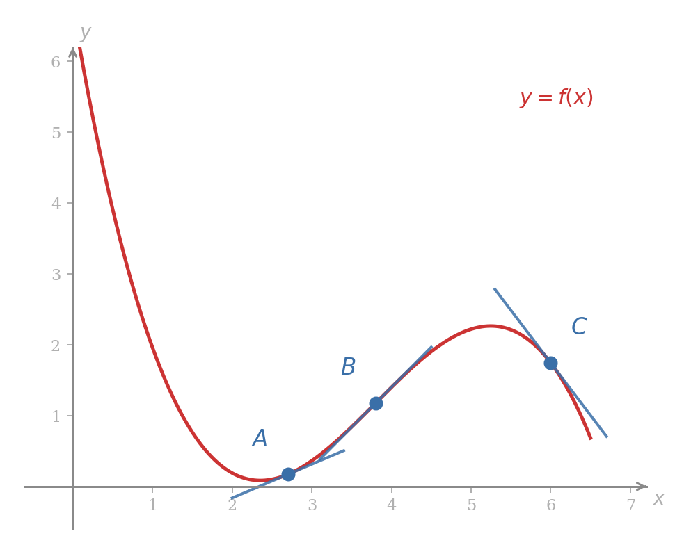
A smooth curve y = f(x) drawn on the plane, with three points marked on it: A on a gently rising stretch, B on a steeply rising stretch further to the right, and C on a falling stretch. Short tangent-like segments at each point indicate the local steepness, with B's segment steeper than A's and C's tilted downward.

The graph above makes the point unmistakable. At $A$ the curve is rising, but only gently; at $B$ , further along, it is rising much more steeply; at $C$ it is falling. The eye reads three distinct rates of change at three distinct points of one and the same function. We have neither a definition that covers them nor a number to attach to any one of them; only the linear-case definition, which fails as soon as we drop linearity.

The way out is to look at two points on the graph rather than one. Through any pair of distinct points on the graph of $f$ there passes a unique straight line, and that line, being linear, has a slope to which the previous reading applies. Taking the two points to be $(x_0, f(x_0))$ and $(x_0 + h, f(x_0 + h))$ and computing the slope by rise over run gives

\frac{f(x_0 + h) - f(x_0)}{h},

the difference quotient introduced at the close of the PM lesson. The smaller the gap $h$ between the two points, the more the connecting line resembles whatever line we would draw to capture the steepness of the graph at $x_0$ alone.

Remark

The intuition is that as $h$ shrinks towards zero the difference quotient should approach a single number describing the steepness of $f$ at $x_0$ . To make this precise we need a way to talk about the value an expression approaches as one of its inputs is sent to a limiting position, even when substituting the limiting value directly is not permitted; here $h = 0$ is forbidden because the difference quotient divides by $h$ . The tool that supplies this is the limit, taken up by a coming lesson. Before approaching it, we settle a handful of properties of the slope that the limit argument and most subsequent calculations will rely on.

Properties of the Slope of a Line

Five properties of the slope recur throughout the course; together they amount to the whole working theory of straight lines on which the limit construction will sit. We collect the statements first, demonstrate each in a short example, and verify them at the end of the section.

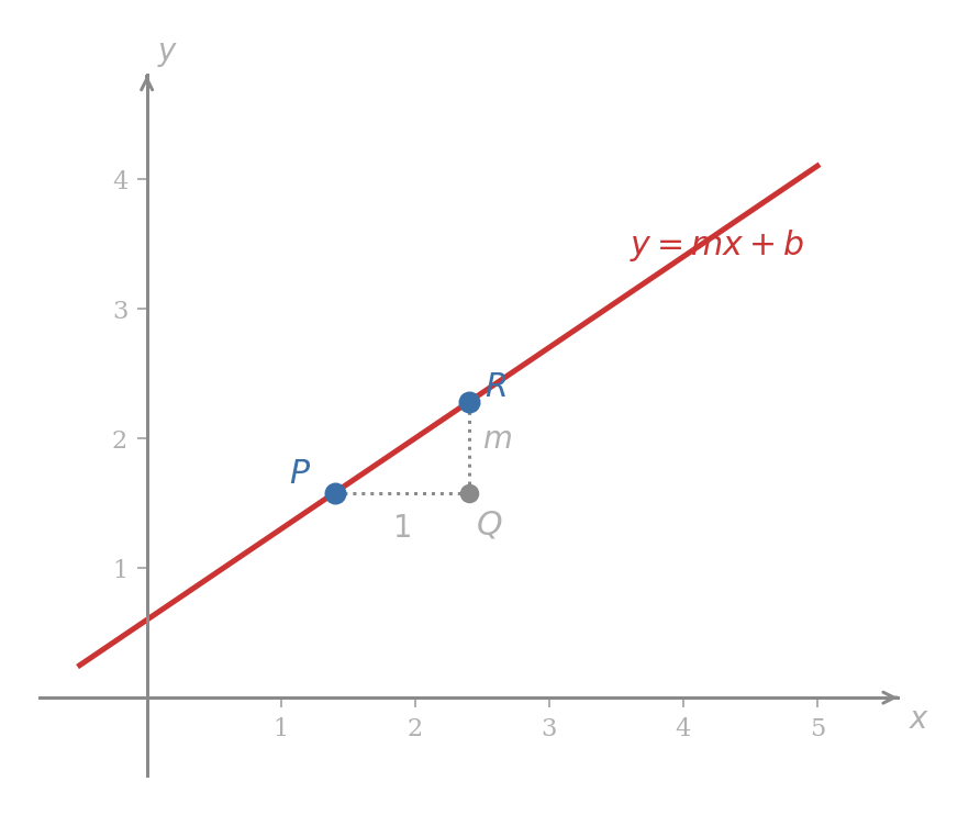
Note (Slope Property 1 (unit-step rule))

Starting from any point on a line of slope $m$ and moving one unit to the right, returning to the line requires moving exactly $m$ units in the vertical direction.

This is the geometric content the AM linear function definition recorded as “each unit step in $x$ raises $y$ by exactly $m$ ”; it is restated here as a property of the line so that the verifications can speak about it cleanly.

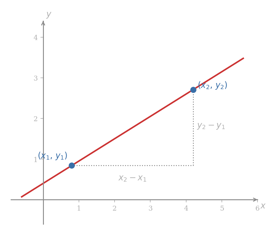
A non-vertical line of slope m drawn in the plane. A point P on the line is marked, a horizontal dotted segment of length one runs from P to the right, ending at an auxiliary point Q below the line, and a vertical dotted segment of length m rises from Q to a point R back on the line. The horizontal step is labelled 1 and the vertical step is labelled m.

Note (Slope Property 2 (two-point formula))

For two distinct points $(x_1, y_1)$ and $(x_2, y_2)$ on a non-vertical line of slope $m$ ,

m = \frac{y_2 - y_1}{x_2 - x_1}.

The right-hand side is unchanged on swapping the roles of the two points: both numerator and denominator change sign together.

A non-vertical line drawn through two marked points (x1, y1) on the left and (x2, y2) on the right. A horizontal dotted segment runs from (x1, y1) rightwards to a corner directly below (x2, y2) labelled with the run x2 minus x1, and a vertical dotted segment rises from that corner up to (x2, y2) labelled with the rise y2 minus y1, the two segments forming a right-triangle whose hypotenuse is the segment of the line.

Note (Slope Property 3 (point-slope form))

A non-vertical line of slope $m$ passing through the point $(x_1, y_1)$ has the equation

y - y_1 = m\,(x - x_1).

This equation is the point-slope form of the line.

Note (Slope Property 4 (parallels))

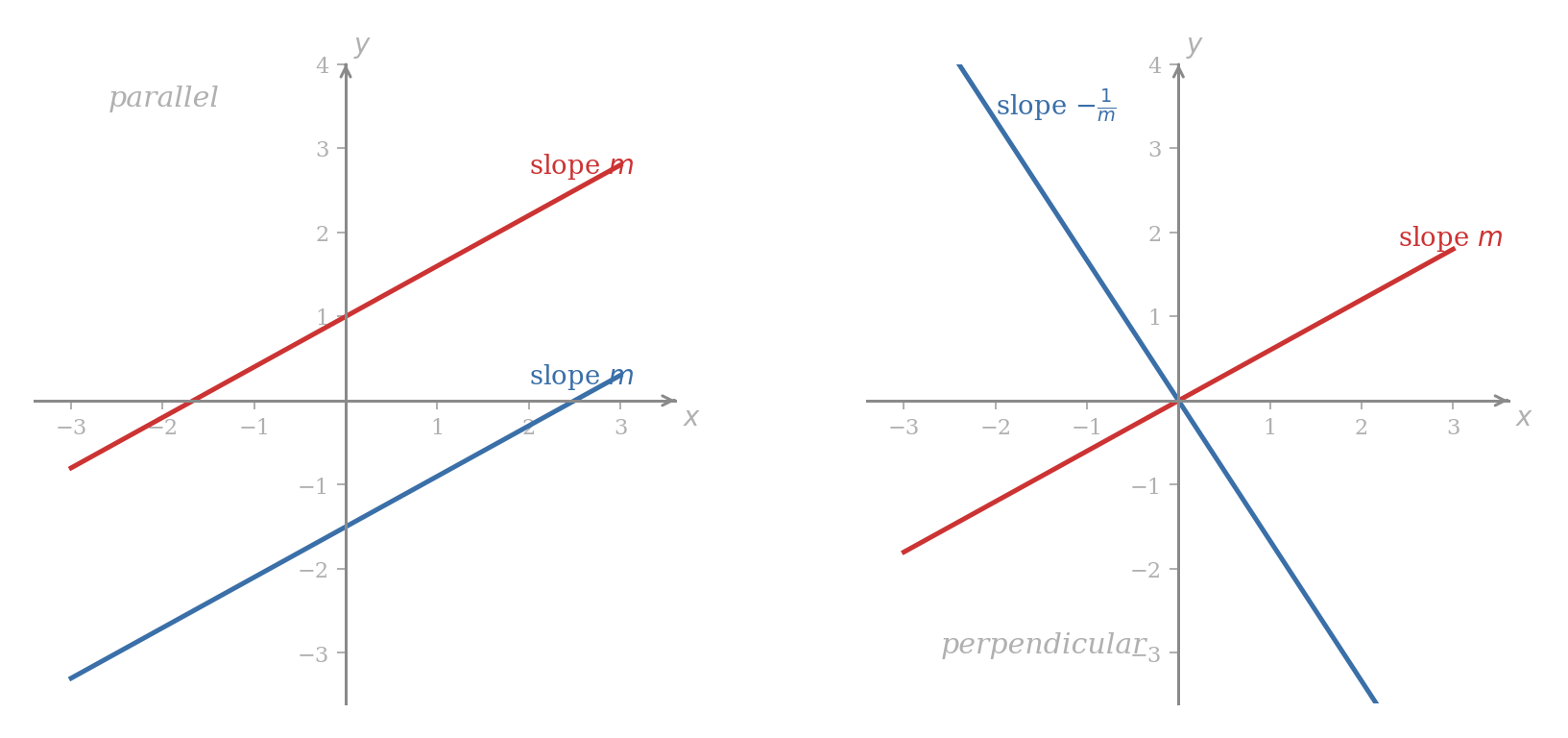
Two distinct non-vertical lines are parallel if and only if they have the same slope.

Note (Slope Property 5 (perpendiculars))

Two non-vertical and non-horizontal lines are perpendicular if and only if the product of their slopes is $-1$ .

Two side-by-side panels. The left panel shows two parallel lines of the same slope m, drawn one above the other, labelled parallel. The right panel shows two lines through the origin meeting at right angles, the first of slope m rising gently and the second of slope minus one over m falling steeply, labelled perpendicular.

Calculations using the properties

Example 42 (Slope and

y

-intercept from a general equation)

Find the slope and $y$ -intercept of the line $4x - 5y = 20$ .

The line is non-vertical because the coefficient of $y$ is non-zero, so we may put the equation in the slope-intercept form of the AM lesson by isolating $y$ ,

-5y = 20 - 4x, \qquad y = \tfrac{4}{5} x - 4.

The slope is $\tfrac{4}{5}$ and the $y$ -intercept is $(0, -4)$ .

Example 43 (Sketching from a point and a slope)

Sketch the line of slope $2$ through $(3, -2)$ .

By slope property 1, starting at $(3, -2)$ and moving one unit right lands at $(4, -2)$ , off the line by an amount equal to the slope; moving $2$ units upwards from there lands at $(4, 0)$ , which is on the line. The line is then drawn through $(3, -2)$ and $(4, 0)$ .

The same procedure with the slope $-\tfrac{3}{4}$ through $(-1, 4)$ proceeds identically: from $(-1, 4)$ a unit step right reaches $(0, 4)$ , and a vertical move of $-\tfrac{3}{4}$ reaches $(0, \tfrac{13}{4})$ , the second point used to draw the line.

Two lines drawn on the same set of axes. The first, in red, has slope two and passes through the marked point (3, -2), with a small dotted right-triangle showing the unit step right and the two-unit step up to the line. The second, in blue, has slope negative three quarters and passes through the marked point (-1, 4), with a small dotted right-triangle showing the unit step right and the three-quarter unit step down to the line.

Problem 26

Sketch the line of slope $-2$ through $(-3, 1)$ by the unit-step procedure of slope property 1, identify a second point on the line by the same construction, and write the line in the form $y = mx + b$ .

Example 44 (Slope through two given points)

Find the slope of the line through $(-3, 5)$ and $(4, -2)$ .

By slope property 2 with $(x_1, y_1) = (-3, 5)$ and $(x_2, y_2) = (4, -2)$ ,

m = \frac{-2 - 5}{4 - (-3)} = \frac{-7}{7} = -1.

Reversing the labelling produces the same value, $\tfrac{5 - (-2)}{-3 - 4} = \tfrac{7}{-7} = -1$ , in line with the symmetry noted alongside Property 2.

Problem 27

Find the slope of the line through $(-2, 7)$ and $(5, -8)$ , and confirm that swapping the two points produces the same value.

Example 45 (Equation from a point and a slope)

Find an equation of the line of slope $2$ through $(4, -3)$ .

Slope property 3 with $m = 2$ and $(x_1, y_1) = (4, -3)$ gives

y - (-3) = 2\,(x - 4), \qquad \text{that is,} \qquad y + 3 = 2x - 8.

The slope-intercept form follows by isolating $y$ , namely $y = 2x - 11$ .

Example 46 (Equation through two points)

Find an equation of the line through $(2, 1)$ and $(-1, 7)$ .

Slope property 2 furnishes the slope first,

m = \frac{7 - 1}{-1 - 2} = \frac{6}{-3} = -2,

and slope property 3 with the first point completes the equation,

y - 1 = -2\,(x - 2), \qquad \text{that is,} \qquad y = -2x + 5.

A check using the second point: $-2 \cdot (-1) + 5 = 7$ , as required.

Problem 28

Find an equation of the line through $(0, -3)$ and $(4, 5)$ in slope-intercept form, and verify your answer by substituting both given points back into it.

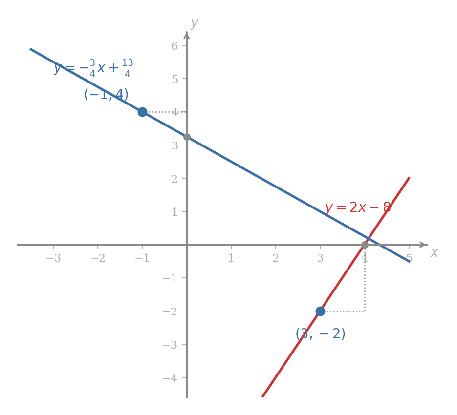
Example 47 (A line parallel to a given line)

Find an equation of the line through $(1, -2)$ parallel to $3x - 4y = 12$ .

First put the given line in slope-intercept form: $-4y = 12 - 3x$ , so $y = \tfrac{3}{4} x - 3$ , of slope $\tfrac{3}{4}$ . Slope property 4 says any line parallel to it has the same slope, and slope property 3 then gives

y - (-2) = \tfrac{3}{4}\,(x - 1), \qquad \text{that is,} \qquad y = \tfrac{3}{4} x - \tfrac{11}{4}.

Example 48 (A perpendicular line)

Find an equation of the line through $(2, 5)$ perpendicular to $y = \tfrac{1}{3} x + 4$ .

The given line has slope $\tfrac{1}{3}$ . By slope property 5 the perpendicular slope $m$ satisfies $\tfrac{1}{3} \cdot m = -1$ , hence $m = -3$ . Slope property 3 then supplies

y - 5 = -3\,(x - 2), \qquad \text{that is,} \qquad y = -3x + 11.

Problem 29

Find an equation of the line through $(-4, 1)$ that is perpendicular to $2x + 3y = 9$ , and confirm by computing the product of the two slopes that slope property 5 holds.

Problem 30

For each of the lines below, state the slope and the $y$ -intercept.

$5x + 2y = 8$ .
$y = 4 - 7x$ .
The line through $(0, -1)$ and $(3, 5)$ .
The line through $(-2, 4)$ parallel to $y = -\tfrac{1}{2} x + 9$ .

Slope as a Rate of Change Across an Interval

The previous section read the slope of $L(x) = mx + b$ as the unit-step rate of change. Slope property 2 upgrades this reading to arbitrary intervals: for $x_1 \neq x_2$ , as $x$ runs from $x_1$ to $x_2$ , the value of $L$ runs from $y_1 = L(x_1)$ to $y_2 = L(x_2)$ , and the rate of change of $L$ over the interval is

\frac{L(x_2) - L(x_1)}{x_2 - x_1} = \frac{y_2 - y_1}{x_2 - x_1} = m

by slope property 2. The slope is therefore the rate of change of $L$ over every interval, not only over a unit step. This constancy across all intervals is what makes a function linear; later lessons take up what happens when it fails.

Example 49 (A descending aircraft)

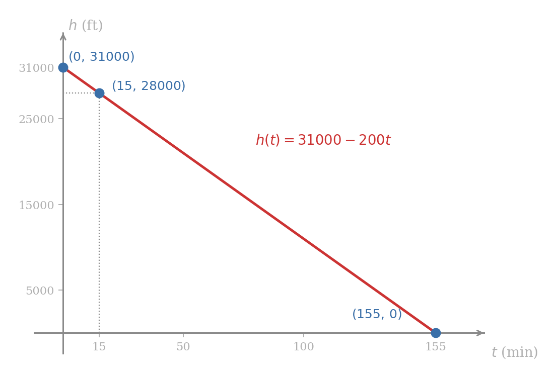
An airliner descends at a constant rate. Air traffic records show that at fifteen minutes into the descent the aircraft is at $28{,}000$ feet, and the descent rate is $200$ feet per minute. Writing $t$ for the number of minutes since the descent began and $h(t)$ for the altitude, the constancy of the rate makes $h$ a linear function with slope $-200$ , so $h(t) = -200 t + b$ for some constant $b$ . Substituting the recorded value $h(15) = 28{,}000$ ,

-200 \cdot 15 + b = 28{,}000, \qquad \text{so} \qquad b = 31{,}000,

and the altitude function is $h(t) = 31{,}000 - 200 t$ . The starting altitude was $h(0) = 31{,}000$ feet, and the aircraft will reach the ground at the input $t$ for which $h(t) = 0$ , that is at $t = 155$ minutes.

The graph of the altitude function h(t) = 31000 - 200t for t between 0 and 155 minutes, falling linearly from the y-intercept (0, 31000) through the marked point (15, 28000) and down to the x-intercept (155, 0). Dotted lines drop from the (15, 28000) point to both axes.

Problem 31

A storage cylinder of liquid nitrogen evaporates at a constant rate. At three hours past the start of an experiment the cylinder holds $42$ litres, and at seven hours past the start it holds $34$ litres. Find the volume $V(t)$ as a linear function of the time $t$ in hours, identify the time at which the cylinder is empty, and state the volume at $t = 0$ .

Verification of the properties

The verifications proceed in the order $2$ , $3$ , $1$ , $4$ , $5$ . The first three are pure algebra from the slope-intercept form; the last two require a small piece of plane geometry.

Note (Pythagoras (used below))

We use the Pythagorean theorem and its converse: in a right triangle with legs of lengths $a$ and $b$ and hypotenuse of length $c$ , one has $a^2+b^2=c^2$ , and conversely if $a^2+b^2=c^2$ then the angle opposite the side of length $c$ is a right angle. In the proof below we write $|PQ|$ for the length (distance) of the segment joining two points $P$ and $Q$ .

Proof

Property 2. Let the non-vertical line have equation $y = mx + b$ , and let $(x_1, y_1)$ and $(x_2, y_2)$ be two distinct points on it. Then $y_1 = m x_1 + b$ and $y_2 = m x_2 + b$ , and subtracting,

y_2 - y_1 = m\,(x_2 - x_1).

The two points being distinct on a non-vertical line forces $x_1 \neq x_2$ , since equal $x$ -coordinates would force equal $y$ -coordinates by the slope-intercept formula. Dividing by $x_2 - x_1$ ,

\frac{y_2 - y_1}{x_2 - x_1} = m,

which is the claim.

■

Proof

Property 3. Rewriting $y - y_1 = m(x - x_1)$ as

y = m x + (y_1 - m x_1)

shows it is in slope-intercept form, with slope $m$ and $y$ -intercept $(0,\, y_1 - m x_1)$ , so it describes a line of slope $m$ . Substituting $x = x_1$ gives $y = m x_1 + y_1 - m x_1 = y_1$ , so the point $(x_1, y_1)$ lies on this line. A line of slope $m$ is determined by any one of its points, so this is the unique such line through $(x_1, y_1)$ .

■

Proof

Property 1. Let the line have slope $m$ and let $P = (x_1, y_1)$ be a point on it. The point $Q$ obtained from $P$ by moving one unit to the right has coordinates $(x_1 + 1, y_1)$ , and we look for the height $y_2$ at which the line crosses the vertical line $x = x_1 + 1$ . By slope property 2 applied to the points $(x_1, y_1)$ and $(x_1 + 1, y_2)$ ,

m = \frac{y_2 - y_1}{(x_1 + 1) - x_1} = y_2 - y_1.

Hence $y_2 - y_1 = m$ , which is the vertical displacement from $Q$ to the line, as claimed.

■

Proof

Property 4. Let two distinct non-vertical lines have equations $y = m_1 x + b_1$ and $y = m_2 x + b_2$ . They are parallel exactly when they fail to intersect, that is, exactly when the equation

m_1 x + b_1 = m_2 x + b_2

has no solution in $x$ . Rearranging gives $(m_1 - m_2)\,x = b_2 - b_1$ . If $m_1 \neq m_2$ the equation has the unique solution $x = (b_2 - b_1)/(m_1 - m_2)$ , so the lines do meet, contradicting parallelism. If $m_1 = m_2$ then the equation collapses to $0 = b_2 - b_1$ ; this holds for some $x$ only when $b_1 = b_2$ , in which case the two lines coincide and are not distinct. The remaining case $m_1 = m_2$ with $b_1 \neq b_2$ leaves the equation with no solution, and the lines are parallel. Thus distinct non-vertical lines are parallel exactly when their slopes coincide.

■

Proof

Property 5. Shifting both lines by the same horizontal and vertical amounts changes neither the slopes nor the angle between them, so we may shift each line so that it passes through the origin without altering perpendicularity or slope. Assume then that both lines pass through the origin with slopes $m_1$ and $m_2$ , neither vertical nor horizontal, so $m_1$ and $m_2$ are finite and non-zero. The first line contains the point $A = (1, m_1)$ and the second contains $B = (1, m_2)$ , and both lines pass through $O = (0, 0)$ . The triangle $OAB$ has a right angle, if anywhere, at $O$ , since the sides $OA$ and $OB$ lie along the two lines that meet there. By the converse of Pythagoras’ theorem the triangle is right-angled at $O$ exactly when

|OA|^2 + |OB|^2 = |AB|^2.

Each squared side length is computed by Pythagoras on a right triangle with axis-parallel legs: from $O$ to $(1, 0)$ to $A$ gives $|OA|^2 = 1 + m_1^2$ , the same construction with $B$ in place of $A$ gives $|OB|^2 = 1 + m_2^2$ , and since $A$ and $B$ share the same $x$ -coordinate, $|AB|^2 = (m_1 - m_2)^2$ . Substituting,

(1 + m_1^2) + (1 + m_2^2) = m_1^2 - 2 m_1 m_2 + m_2^2,

which simplifies to $2 = -2 m_1 m_2$ , that is, $m_1 m_2 = -1$ . The converse retraces the same identity backwards, so $m_1 m_2 = -1$ if and only if the lines are perpendicular.

■

The Slope of a Curve at a Point

Two of the readings established for a line, the rise-over-run formula and the rate-of-change interpretation, both depend on the line having a single slope. A curve has no single slope. The first task of this section is to attach a slope to a curve at one of its points; the second is to read that number, when it is available, as a rate of change at that point.

Tangent line at a point

The geometric idea is most familiar in the case of a circle. A line is tangent to a circle at a point $P$ if it meets the circle only at $P$ , leaving the circle entirely on one side. Looking at a small region around $P$ , the circle bends so gently that it is hard to distinguish from the tangent line itself; on closer inspection the circle bends a little, but increasing the magnification reduces the discrepancy without bound.

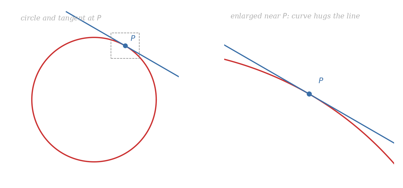
Two side-by-side panels. The left panel shows a full circle with a straight line drawn tangent to it at a marked point P, and a dashed rectangle drawn around P highlighting a small region. The right panel shows the same point P at higher magnification: only a short arc of the circle and the same tangent line remain in view, and the arc visibly hugs the line.

The same picture works for a smooth curve that is not a circle, provided the curve has a definite direction at $P$ . Zooming in repeatedly on a small region around $P$ makes the curve look straighter; under sufficiently strong magnification the curve becomes indistinguishable, on the screen, from a single straight line. This line is what we mean by the tangent line to the curve at $P$ .

Definition 20 (Tangent Line, Slope of a Curve)

The tangent line to a curve at a point $P$ on it is the straight line through $P$ that the curve approaches under successively higher magnification near $P$ . When this tangent line has a slope, the slope of the curve at $P$ is defined to be the slope of its tangent line at $P$ .

The phrase “approaches under successively higher magnification” carries the same intuition the difference quotient of the previous section gestured at: as the second point on the curve moves towards $P$ , the line through the two points approaches the tangent line. A coming lesson will replace this intuition with a precise construction by means of the limit, but the geometry is enough for the present section, in which we work from pictures and from one closed formula.

A curve does not always carry a tangent line. The absolute value graph $y = |x|$ from the PM lesson has a sharp corner at the origin: zooming in on $(0, 0)$ never makes the corner straighten out, and no single line approximates the graph there. We will keep silent about such points until the limit machinery lets us speak of them precisely.

Reading slopes off a graph

When the tangent line is drawn on a graph, its slope can often be read directly by slope property 1 of the previous section: starting from the point of tangency, move one unit to the right and observe the vertical shift back to the line.

Example 50 (The slope of

y = x^2

(1, 1)

)

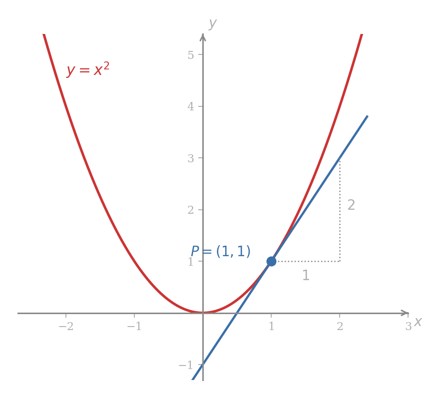
The graph of $y = x^2$ and its tangent line at the point $P = (1, 1)$ are shown below. From the figure, a unit step to the right of $P$ takes the tangent line up by exactly $2$ units, so by slope property 1 the tangent slope is $2$ , and the slope of the curve $y = x^2$ at $P$ is therefore $2$ as well.

The parabola y = x squared with its tangent line drawn at the point P = (1, 1). A small dotted right-triangle attached to the tangent line shows a unit step right from P labelled 1 and a vertical step up labelled 2, illustrating that the tangent line has slope 2.

Problem 32

The tangent line to the graph of a function $g$ at the point $P = (-2, 3)$ is drawn alongside the graph and is observed to fall by $5$ units for every $2$ units of rightward motion. State the slope of $g$ at $P$ and give an equation for the tangent line in point-slope form.

The slope as an instantaneous rate of change

The previous section read the slope of a linear function as its rate of change, valid at every input because of constancy. For a curve, the slope at $P$ is defined as the slope of the tangent line at $P$ , and the tangent line is precisely the linear approximation of the curve near $P$ . Replacing the curve by its tangent line near $P$ , the same rate-of-change reading carries through, but now restricted to the single input $P$ .

Definition 21 (Instantaneous Rate of Change)

The instantaneous rate of change of a function $f$ at a point $P$ on its graph is the slope of the curve $y = f(x)$ at $P$ , that is, the slope of the tangent line at $P$ when that tangent line has a slope.

For a linear function the instantaneous rate of change at every input equals the slope $m$ , recovering the previous section’s definition. For a curve, the instantaneous rate of change varies from point to point and records how fast the function is changing at each individual input.

Example 51 (Instantaneous fuel consumption)

A hospital’s emergency diesel generator runs through a $24$ -hour period of heavy load, with its consumption monitored by a precision flow meter. Writing $t$ for the time in hours since midnight and $V(t)$ for the volume of fuel in the tank in litres, the recorded curve is non-linear: the generator burns fuel faster during peak operating hours than during quieter ones. The point $P$ marks the volume at $7{:}30$ a.m.

A non-linear curve representing the volume of fuel V in litres in a generator tank as a function of time t in hours over a single 24-hour day. The curve falls overall but with varying steepness, dropping faster around the middle of the day and slower at the ends; a marked point P sits on the curve at about t = 7.5 hours, and the tangent line drawn at P slopes downwards with a clearly negative slope.

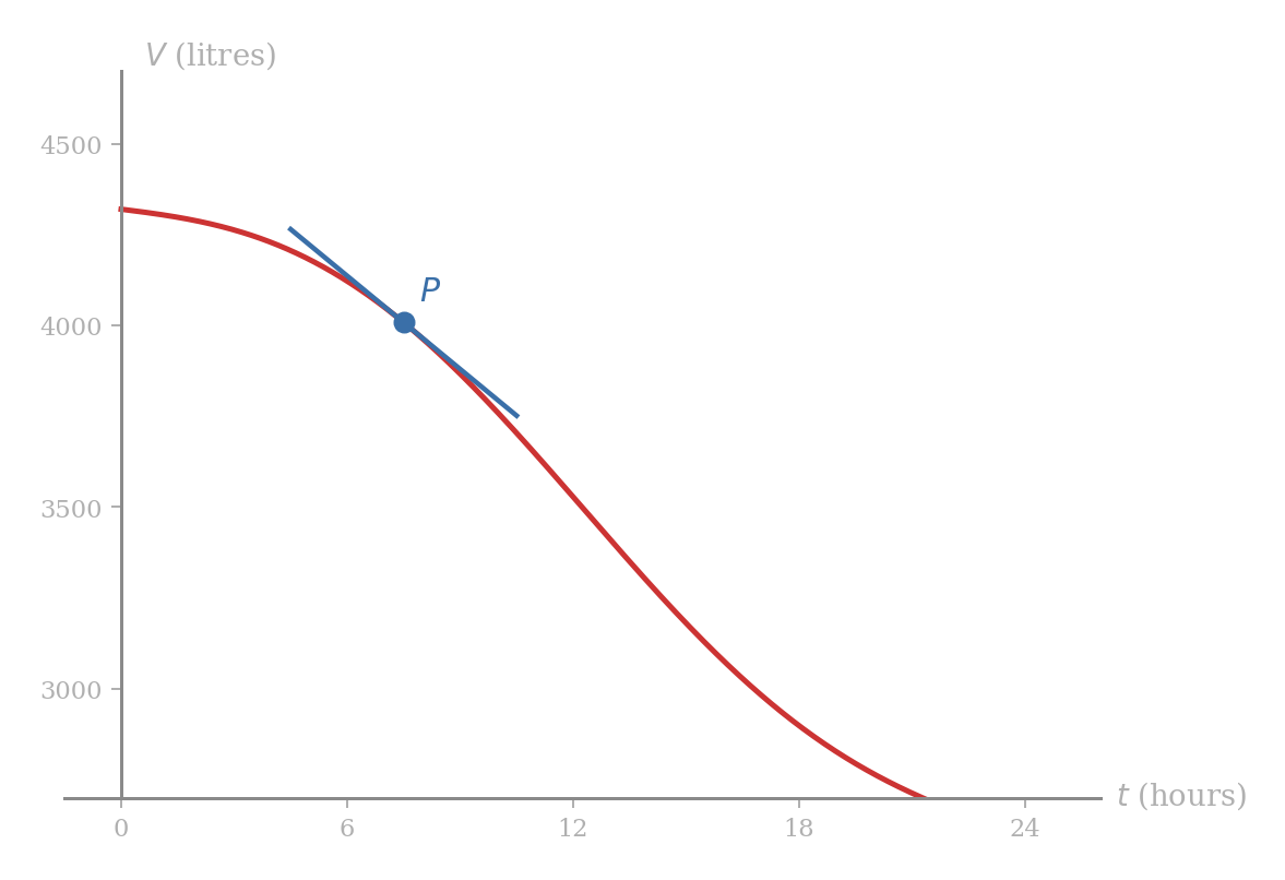
The tangent at $P$ falls clearly. Reading its slope off the figure as approximately $-85$ litres per hour, the generator is consuming fuel at about $85$ litres per hour at that instant. At a quieter hour the tangent would be shallower and the instantaneous rate smaller; at noon, when the curve is at its steepest in the figure, the tangent slope is more negative still and the rate correspondingly larger. A linear model would replace the entire curve by a single straight line of constant slope and report only the average over the day, losing this detail.

Problem 33

A car’s odometer is recorded continuously during a journey and produces a graph of distance against time on which the slope at any point of the curve gives the speed of the car at that instant. If the tangent line at the point $P = (40, 30)$ , where time is measured in minutes and distance in kilometres, has slope $\tfrac{3}{4}$ , state the speed of the car at the recorded instant in kilometres per minute and convert the answer to kilometres per hour.

A slope formula for $y = x^2$

Reading slopes off a graph by eye is the right place to start, but it is too imprecise to be useful when the slope is needed at many points at once. For most curves the slope at each point can be packaged in a single closed formula; the derivation belongs to a coming lesson, but the formula for the simplest curved graph, the parabola $y = x^2$ , is worth stating and using now.

Theorem 3 (Slope of

y = x^2

)

The slope of the parabola $y = x^2$ at the point $(a, a^2)$ is $2a$ . Equivalently, the tangent line to $y = x^2$ at $(a, a^2)$ has slope $2a$ and equation

y - a^2 = 2a\,(x - a).

The proof is deferred to a coming lesson, where the limit construction needed to obtain it will be in place.

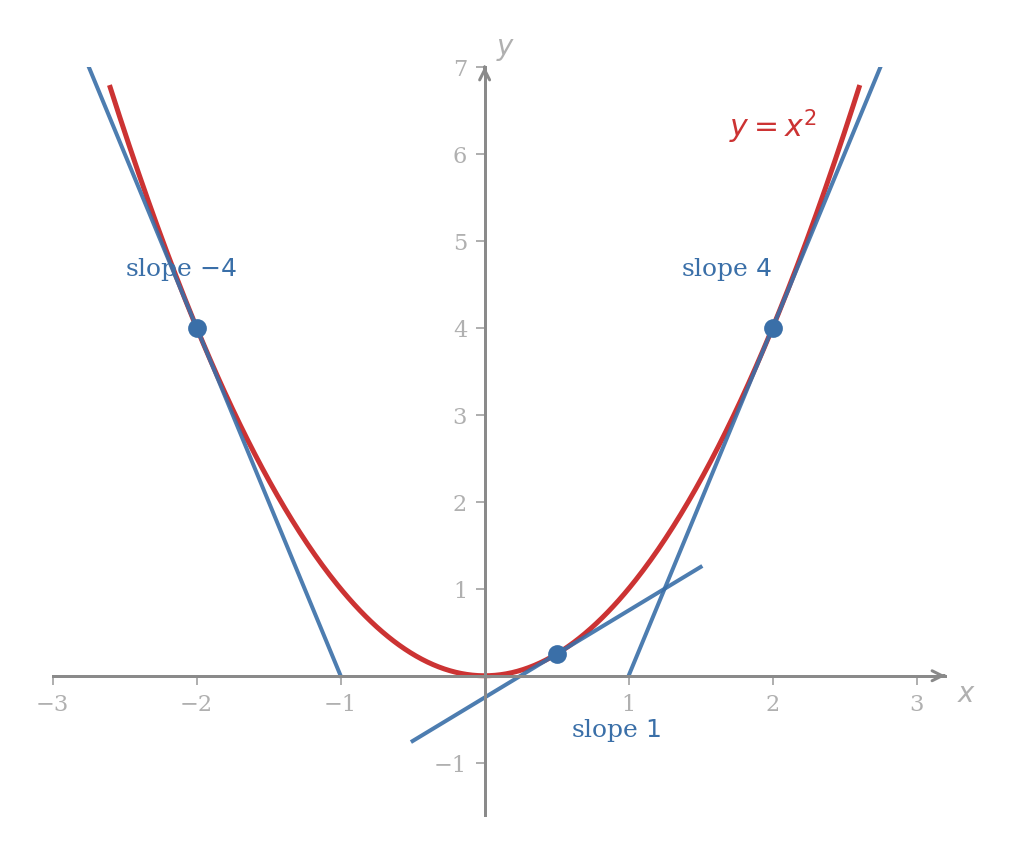
The formula is consistent with the picture: at $a = 1$ it returns slope $2$ , agreeing with the previous example; at $a = 0$ it returns slope $0$ , agreeing with the horizontal tangent at the vertex of the parabola; for $a < 0$ it returns a negative slope, agreeing with the left branch descending toward the vertex.

The parabola y = x squared drawn with three short tangent line segments at three marked points: at (-2, 4) the tangent has slope -4, at (1/2, 1/4) the tangent has slope 1, and at (2, 4) the tangent has slope 4, illustrating that the slope at the point with x-coordinate a is 2a.

Example 52 (Using the slope formula)

Find the slope of $y = x^2$ at the point $\left(\tfrac{3}{2}, \tfrac{9}{4}\right)$ , and write an equation for the tangent line at that point.

The $x$ -coordinate of the point is $a = \tfrac{3}{2}$ , so the slope formula gives slope $2 \cdot \tfrac{3}{2} = 3$ . By slope property 3 of the previous section, the tangent line in point-slope form is

y - \tfrac{9}{4} = 3\,(x - \tfrac{3}{2}),

or, isolating $y$ , $y = 3x - \tfrac{9}{4}$ .

Example 53 (A horizontal tangent)

The slope formula gives $0$ at $a = 0$ , so the tangent line to $y = x^2$ at the origin is horizontal, with equation $y = 0$ . Geometrically, the parabola has its vertex at the origin and the horizontal axis just grazes it there, in agreement with the unit-step picture: any unit step from $(0, 0)$ along the tangent leaves $y$ unchanged.

Problem 34

For the parabola $y = x^2$ :

Find the slope at the points $(-3, 9)$ , $\left(\tfrac{1}{4}, \tfrac{1}{16}\right)$ , and $(5, 25)$ .
Write an equation of the tangent line to $y = x^2$ at the point $(-1, 1)$ in point-slope form, and convert it to slope-intercept form.
At which point of the parabola is the tangent line parallel to the line $y = 4x - 7$ ?

Video

Lesson assets

Slopes and Rates of Change

Rates of Change

Properties of the Slope of a Line

Calculations using the properties

Slope as a Rate of Change Across an Interval

Verification of the properties

The Slope of a Curve at a Point

Tangent line at a point

Reading slopes off a graph

The slope as an instantaneous rate of change

A slope formula for y=x2y = x^2y=x2

A slope formula for $y = x^2$