20/02/2026

#Math#Differentiation

Lesson assets

No linked assets.

Rules for Differentiation

Lesson 2PM verified the power rule for several special exponents and stated it for every rational $r$ , but the Rule reaches only the bare power function $x^{r}$ . Most functions of interest in this course are built from such powers by two further operations: multiplication by a constant, as in $7 x^{4}$ , and addition, as in $x^{3} + 5 x - 2$ . Each operation interacts with differentiation in a way fixed by the limit definition itself, and the resulting two rules are enough to differentiate every polynomial by inspection. A third rule, generalising the power rule from $x$ to an arbitrary differentiable expression $g(x)$ , is recorded at the end of the section for use later in the course.

The constant multiple rule

Theorem 1 (Constant-Multiple Rule)

Let $f$ be differentiable at $x$ in the sense of Lesson 2PM, and let $k$ be a real number independent of $x$ . Then $kf$ is differentiable at $x$ and

\frac{d}{dx}\bigl(k\,f(x)\bigr) = k \cdot \frac{d}{dx}\,f(x).

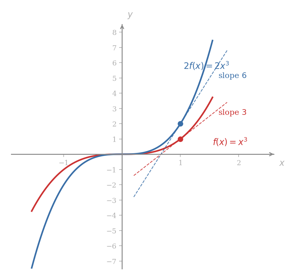
A constant multiplier rides along through differentiation, untouched. The factor $k$ scales the rise of every secant of $f$ by exactly the same amount $k$ without altering its run, so the slope of every secant of $kf$ is $k$ times the slope of the corresponding secant of $f$ , and the same factor survives the limit. The verification at the end of the section makes the remark precise.

Example 1 (A constant multiplier on a single power)

For $f(x) = 7 x^{4}$ take $k = 7$ and the inner function $x^{4}$ , whose derivative is $4 x^{3}$ by the power rule of Lesson 2PM. The constant multiple rule then gives

f'(x) = 7 \cdot \frac{d}{dx}\bigl(x^{4}\bigr) = 7 \cdot 4 x^{3} = 28 x^{3}.

The same step handles a negative scalar without ceremony: $\frac{d}{dx}\bigl(-\tfrac{1}{3} x^{5}\bigr) = -\tfrac{5}{3} x^{4}$ .

The cubic curve y equals x cubed drawn alongside its vertical scaling y equals 2 x cubed in a contrasting colour. At the point with x equal to 1 each curve carries a short dashed tangent segment, the lower one labelled with slope 3 and the upper one with slope 6, illustrating that vertical scaling by 2 doubles the slope of the tangent at every point.

Example 2 (Carrying a fractional multiplier through a root)

For $f(x) = \tfrac{2}{5} \sqrt{x}$ on $x > 0$ , write $\sqrt{x} = x^{1/2}$ as in Recitation 1 and apply the power rule with $r = \tfrac{1}{2}$ ,

f'(x) = \tfrac{2}{5} \cdot \frac{d}{dx}\bigl(x^{1/2}\bigr) = \tfrac{2}{5} \cdot \tfrac{1}{2} x^{-1/2} = \frac{1}{5\sqrt{x}}.

The constant $\tfrac{2}{5}$ rides along to the end and never participates in the differentiation itself.

Problem 1

Compute the derivative of each function below by the constant multiple rule and the power rule, stating the inputs at which the derivative is defined.

$f(x) = 9 x^{6}$ .
$f(x) = -\tfrac{1}{2} x^{-3}$ .
$f(x) = 4 / x^{2}$ .
$f(x) = -\tfrac{3}{4} x^{2/3}$ .

The Sum Rule

Theorem 2 (Sum Rule)

Let $f$ and $g$ be differentiable at $x$ in the sense of Lesson 2PM. Then $f + g$ is differentiable at $x$ and

\frac{d}{dx}\bigl(f(x) + g(x)\bigr) = \frac{d}{dx}\,f(x) + \frac{d}{dx}\,g(x).

The same identity, with the sign of the second term reversed throughout, gives the difference rule

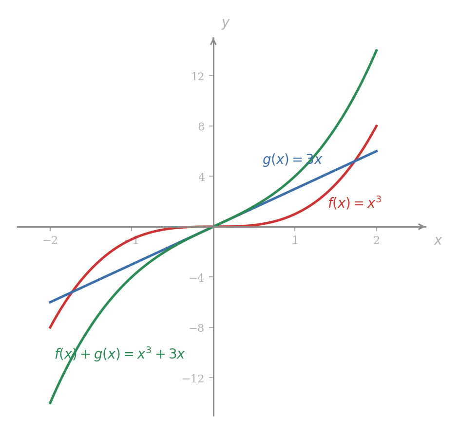
\frac{d}{dx}\bigl(f(x) - g(x)\bigr) = \frac{d}{dx}\,f(x) - \frac{d}{dx}\,g(x).

The derivative of a sum is the sum of the derivatives, and the same is true for differences. Applied to a polynomial term by term, the sum rule together with the constant multiple rule and the power rule reduces every differentiation to the mechanical procedure of dropping each exponent by one and bringing it round to the front.

Example 3 (Differentiating a polynomial term by term)

For $f(x) = 2 x^{4} - 5 x^{3} + x - 7$ the Sum and Difference Rules apply across the four terms, the constant multiple rule strips each leading coefficient, and the power rule handles each remaining power. The constant term contributes $0$ by the constant case from Lesson 2PM, so

f'(x) = 2 \cdot 4 x^{3} - 5 \cdot 3 x^{2} + 1 \cdot 1 - 0 = 8 x^{3} - 15 x^{2} + 1.

With practice the intermediate steps fold into a single line of writing, and the derivative of any polynomial is read off by inspection.

Three curves drawn on a single set of axes: the cubic y equals x cubed, the line y equals 3 x, and the sum y equals x cubed plus 3 x. The sum curve sits above the cubic for positive x by exactly the height of the line, and below it for negative x by the same amount, showing that the graph of f plus g is obtained by stacking the heights of f and g vertically.

Example 4 (A sum of non-integer powers)

For $f(x) = 6 \sqrt{x} + 3 / x$ on $x > 0$ , rewrite the function in power notation as $6 x^{1/2} + 3 x^{-1}$ and apply the same machinery,

f'(x) = 6 \cdot \tfrac{1}{2} x^{-1/2} + 3 \cdot (-1) x^{-2} = \frac{3}{\sqrt{x}} - \frac{3}{x^{2}}.

Care with the natural domain matches the power rule itself: the first term restricts to $x > 0$ , the second to $x \neq 0$ , and the intersection $(0, \infty)$ is the domain of $f'$ .

Remark (A sum is not a product)

The sum rule splits a derivative across $+$ and $-$ , and across nothing else. The corresponding statement for a product is false: writing $h(x) = x \cdot x = x^{2}$ and treating each factor separately would give $h'(x) = 1 \cdot 1 = 1$ , while the power rule supplies the correct $h'(x) = 2 x$ . Products are governed by a separate rule developed in a later MA0A lesson, and until that rule is in place every product must be either expanded into a sum first, as in $h$ above, or left alone.

Problem 2

Compute the derivative of each function by combining the Sum, Constant-Multiple, and power rules.

$f(x) = x^{5} + 4 x^{3} - 6 x + 2$ .
$f(x) = \tfrac{1}{3} x^{6} - \tfrac{1}{2} x^{4} + 9$ .
$f(x) = 2 x^{1/2} - 5 x^{-1/2}$ .
$f(x) = (x^{2} + 1)(x - 3)$ , by expanding before differentiating.

The General Power Rule

The power rule of Lesson 2PM differentiates $x^{r}$ , the $r$ th power of the bare identity $x$ . When the inner expression is replaced by a more complicated differentiable function $g(x)$ , the form of the answer survives essentially unchanged, with one extra factor.

Theorem 3 (General Power Rule)

Let $g$ be differentiable at $x$ and let $r$ be a rational number for which the power $g(x)^{r}$ is defined on inputs near $x$ and at $x$ itself. Assume also that the outer power function is differentiable at $g(x)$ ; this is automatic when $r$ is a positive integer or when $g(x) > 0$ , but zeros of $g$ require separate checking. Then $g(x)^{r}$ is differentiable at $x$ and

\frac{d}{dx}\bigl(g(x)^{r}\bigr) = r\,g(x)^{r - 1} \cdot \frac{d}{dx}\,g(x).

The proof is deferred to a later MA0A lesson, where the chain-like manipulation needed to obtain it is treated systematically.

The factor $r\,g(x)^{r - 1}$ is the answer the power rule would supply if $g(x)$ were itself the variable; the additional $g'(x)$ corrects for the fact that the inner expression is itself changing with $x$ at its own rate. With $g(x) = x$ the correction collapses to $1$ and the General Rule reduces to the power rule with no information gained; the gain comes when $g$ is genuinely non-trivial.

Example 5 (Verification of the rule on a tractable case)

The Rule was stated without proof, but a small case can be checked directly. Take $f(x) = (x^{2} + 3)^{2}$ , with $g(x) = x^{2} + 3$ and $r = 2$ . The General Rule supplies

f'(x) = 2\,(x^{2} + 3) \cdot 2 x = 4 x\,(x^{2} + 3) = 4 x^{3} + 12 x.

On the other hand, expanding $f$ first as $(x^{2} + 3)^{2} = x^{4} + 6 x^{2} + 9$ and differentiating term by term by the rules of the previous two sections,

f'(x) = 4 x^{3} + 12 x + 0 = 4 x^{3} + 12 x.

The two procedures agree. The expansion method always works for an integer exponent and a polynomial inner function but becomes prohibitive even at modest powers; the General Rule is the closed-form answer to which the binomial expansion would, after pages of arithmetic, eventually collapse.

Example 6 (A power of a binomial)

For $f(x) = (3 x + 5)^{4}$ take $g(x) = 3 x + 5$ and $r = 4$ . The inner derivative is $g'(x) = 3$ by the linear case from Lesson 2PM, and the General Rule gives

f'(x) = 4\,(3 x + 5)^{3} \cdot 3 = 12\,(3 x + 5)^{3}.

Expanding $(3 x + 5)^{4}$ first by the binomial theorem and differentiating term by term reproduces the same answer at greater length; the General power rule packages the entire expansion into a single line.

Example 7 (A fractional power of a quadratic)

For $f(x) = (x^{2} + 1)^{3/2}$ on the whole real line take $g(x) = x^{2} + 1$ and $r = \tfrac{3}{2}$ . The Sum and power rules give $g'(x) = 2 x$ , and the General Rule supplies

f'(x) = \tfrac{3}{2}\,(x^{2} + 1)^{1/2} \cdot 2 x = 3 x \sqrt{x^{2} + 1}.

The base $x^{2} + 1$ is positive at every real $x$ , so the half-power and the derivative are defined throughout.

Example 8 (A negative power of a polynomial)

For $f(x) = 1 / (x^{2} - 4)$ on $|x| \neq 2$ , write $f(x) = (x^{2} - 4)^{-1}$ and apply the General Rule with $r = -1$ and $g'(x) = 2 x$ :

f'(x) = (-1)(x^{2} - 4)^{-2} \cdot 2 x = -\frac{2 x}{(x^{2} - 4)^{2}}.

The natural domain of $f'$ is the same $|x| \neq 2$ that $f$ itself carried, the squaring of the denominator preserving the exclusion.

Example 9 (Combining the Constant-Multiple Rule with the General Power Rule)

For $f(x) = 4\,(2 x^{3} + 1)^{1/2}$ on the inputs at which $2 x^{3} + 1 \geq 0$ , the outermost operation is multiplication by the constant $4$ , and the constant multiple rule pulls it through differentiation untouched. The remaining derivative is supplied by the General Rule with $g(x) = 2 x^{3} + 1$ , $g'(x) = 6 x^{2}$ , and $r = \tfrac{1}{2}$ ,

f'(x) = 4 \cdot \frac{d}{dx}\bigl((2 x^{3} + 1)^{1/2}\bigr) = 4 \cdot \tfrac{1}{2}\,(2 x^{3} + 1)^{-1/2} \cdot 6 x^{2} = \frac{12 x^{2}}{\sqrt{2 x^{3} + 1}}.

The derivative formula is defined only where $2x^{3} + 1 > 0$ ; at the boundary $2x^{3}+1=0$ the original function is defined but the derivative is not. The cancellation of $4 \cdot \tfrac{1}{2}$ to $2$ is part of the calculation; the rules themselves do nothing more than authorise the chain of equalities.

Note (Constant times a power, in a single line)

The combination just performed arises often enough to be worth recording as a single identity. For any constant $k$ , any function $g$ differentiable at $x$ , and any rational $r$ for which $g(x)^{r}$ is defined,

\frac{d}{dx}\bigl(k\,g(x)^{r}\bigr) = k\,r\,g(x)^{r - 1} \cdot g'(x),

the right-hand side reading exactly as the General Rule output with the constant $k$ retained at the front. The identity is a corollary of the Constant-Multiple and General power rules and adds no new content beyond their conjunction; the cost-function example below is one further application of the same line.

Problem 3

Differentiate each function using the General power rule, stating the natural domain of the result.

$f(x) = (x^{3} - 2 x)^{5}$ .
$f(x) = \sqrt{4 x + 1}$ .
$f(x) = (1 - x^{2})^{-1/2}$ .
$f(x) = (x^{2} + x + 1)^{4}$ .

Verifications

The Sum and constant multiple rules follow directly from the limit definition together with two of the limit theorems of Lesson 2PM. The General power rule needs heavier machinery and is left to a later MA0A lesson.

Proof

constant multiple rule. Let $f$ be differentiable at $x$ , with $f'(x) = \lim_{h \to 0} (f(x + h) - f(x))/h$ , and let $k$ be a real number independent of $h$ . The difference quotient of $kf$ at $x$ is

\frac{k\,f(x + h) - k\,f(x)}{h} = k \cdot \frac{f(x + h) - f(x)}{h}

for every $h \neq 0$ , the factor $k$ pulled out by ordinary arithmetic. Limit Theorem I of Lesson 2PM, applied with the difference quotient of $f$ in place of the inner function, gives

\lim_{h \to 0} \frac{k\,f(x + h) - k\,f(x)}{h} = k \cdot \lim_{h \to 0} \frac{f(x + h) - f(x)}{h} = k\,f'(x),

which is the claim.

■

Proof

sum rule. Let $f$ and $g$ be differentiable at $x$ . The difference quotient of $f + g$ at $x$ separates into two pieces by ordinary arithmetic,

\frac{(f + g)(x + h) - (f + g)(x)}{h} = \frac{f(x + h) - f(x)}{h} + \frac{g(x + h) - g(x)}{h},

valid for every $h \neq 0$ . Both summands have a limit as $h \to 0$ , namely $f'(x)$ and $g'(x)$ , and Limit Theorem III of Lesson 2PM gives

\lim_{h \to 0} \frac{(f + g)(x + h) - (f + g)(x)}{h} = f'(x) + g'(x),

which is the claim. The difference rule follows on replacing $g$ by $-g$ and applying the constant multiple rule with $k = -1$ .

■

Applications

With the three rules in hand, every problem from Lesson 2PM that called for a derivative through the limit definition is settled by inspection, and the time freed is spent on the geometry the derivative is meant to capture.

Example 10 (Tangent line to a cubic)

Find the tangent line to $y = x^{3} - 6 x + 4$ at the point with $x = 2$ .

The Sum, Constant-Multiple, and power rules give the derivative in a single line,

f'(x) = 3 x^{2} - 6,

so the slope at $a = 2$ is $f'(2) = 12 - 6 = 6$ . The height there is $f(2) = 8 - 12 + 4 = 0$ , locating the point of contact at $(2, 0)$ . By the equation of the tangent line at $x = a$ from Lesson 2PM, the tangent line is

y - 0 = 6\,(x - 2), \qquad \text{equivalently,} \qquad y = 6 x - 12.

Example 11 (Horizontal tangents on a quartic)

Locate every point at which the curve $y = x^{4} - 4 x^{3}$ has a horizontal tangent.

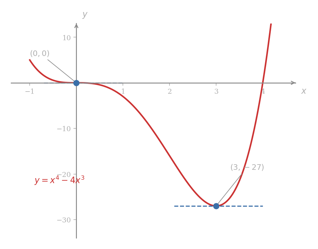
The derivative is $f'(x) = 4 x^{3} - 12 x^{2}$ by the rules of this section, and a horizontal tangent occurs exactly when $f'(x) = 0$ . Factoring,

4 x^{3} - 12 x^{2} = 4 x^{2}\,(x - 3),

the product-zero principle of Recitation 1 gives $x = 0$ or $x = 3$ . The corresponding heights are $f(0) = 0$ and $f(3) = 81 - 108 = -27$ , so the curve has horizontal tangents at $(0, 0)$ and $(3, -27)$ and nowhere else.

The curve y equals x to the fourth minus four x cubed plotted from x slightly less than zero to x just past four, with a dashed horizontal tangent line drawn at the origin and another dashed horizontal tangent drawn at the point with coordinates three and minus twenty-seven. The two tangent points are marked with filled circles, showing the only two locations on this curve where the tangent line is horizontal.

Example 12 (A point with prescribed slope)

Find every point on $y = \sqrt{x}$ at which the tangent line is parallel to $y = \tfrac{1}{6} x + 1$ .

The given line has slope $\tfrac{1}{6}$ , and parallelism by slope property 4 of Lesson 2AM forces the curve to have the same slope at the point of contact. The Constant-Multiple and power rules give

f'(x) = \frac{1}{2 \sqrt{x}}, \qquad x > 0,

and the condition $1/(2 \sqrt{x}) = 1/6$ rearranges to $\sqrt{x} = 3$ , that is $x = 9$ . The single point of contact is $(9, 3)$ , and no other point on the curve has the required slope.

Example 13 (A non-linear refinement of a cost function)

The publisher of Lesson 2AM treated a linear total cost $C(x) = 10{,}000 + 25 x$ , for which the marginal cost is the constant slope $25$ at every production level. A non-linear refinement of the same model replaces $C$ by

C(x) = 100\,(2 x + 25)^{3/2}, \qquad x \geq 0,

where additional production wears the equipment progressively faster. By the constant multiple rule and the General power rule with $g(x) = 2 x + 25$ , $g'(x) = 2$ , and $r = \tfrac{3}{2}$ ,

C'(x) = 100 \cdot \tfrac{3}{2}\,(2 x + 25)^{1/2} \cdot 2 = 300\,\sqrt{2 x + 25}.

The marginal cost is now an increasing function of $x$ , in line with the wear interpretation: the cost of the next copy at production level $x$ exceeds the cost at any lower level. At $x = 0$ the marginal cost is $300 \cdot 5 = 1500$ , and at $x = 12$ it has risen to $300 \cdot 7 = 2100$ , the linear model’s constant $25$ losing all meaning.

Problem 4

For each curve below, compute $f'(x)$ by the rules of this section, then locate every point at which the tangent line is horizontal.

$f(x) = x^{3} - 3 x^{2}$ .
$f(x) = x^{4} - 8 x^{2}$ .
$f(x) = (x^{2} - 1)^{3}$ .

Other Variables and the Second Derivative

The rules above were written in $x$ and $y$ , but the slope formula does not depend on the letters chosen for the input and output. Two minor extensions of the apparatus cover the situations that arise in practice: the input may carry a different name, and the derivative is itself a function and so may be differentiated again.

Independent variables other than $x$

When the input is called $t$ rather than $x$ , the operator $\frac{d}{dx}$ is replaced by $\frac{d}{dt}$ throughout, and the prime notation $f'(t)$ is read as the derivative of $f$ with respect to $t$ . Transferring the slope formula for $x^{2}$ ,

\frac{d}{dt}\bigl(t^{2}\bigr) = 2 t,

the same arithmetic as before with $t$ in place of $x$ . The name of the input alters only the labelling of the axes; the geometry of the slope at a point is unchanged. The slope formula for the cubic, written in any letter,

\frac{d}{du}(u^{3}) = 3 u^{2}, \qquad \frac{d}{ds}(s^{3}) = 3 s^{2}, \qquad \frac{d}{d\theta}(\theta^{3}) = 3 \theta^{2},

records exactly the same statement three times over.

Example 14 (Differentiating with respect to a specific variable)

Compute $\dfrac{d}{dq}\bigl((q^{3} - 2 q + 4)^{7}\bigr)$ .

The General power rule with $g(q) = q^{3} - 2 q + 4$ and $r = 7$ gives

\frac{d}{dq}\bigl((q^{3} - 2 q + 4)^{7}\bigr) = 7\,(q^{3} - 2 q + 4)^{6} \cdot \frac{d}{dq}\bigl(q^{3} - 2 q + 4\bigr) = 7\,(q^{3} - 2 q + 4)^{6}(3 q^{2} - 2),

the inner derivative supplied by the Sum, Constant-Multiple, and power rules in $q$ .

When several letters appear in one expression, the operator $\frac{d}{dt}$ singles out $t$ as the variable and treats every other letter as a constant. The constant multiple rule then carries those letters through differentiation untouched, and the constant case from Lesson 2PM annihilates any term that contains no $t$ at all.

Example 15 (Several letters, one variable)

Compute $\dfrac{d}{dt}\bigl(b\,t^{4} + c\,t^{-2} + d^{3}\bigr)$ , where $b$ , $c$ , $d$ are real numbers independent of $t$ .

Treating $b$ , $c$ , $d$ as constants, the Sum, Constant-Multiple, and power rules apply in turn,

\frac{d}{dt}\bigl(b\,t^{4} + c\,t^{-2} + d^{3}\bigr) = b \cdot 4 t^{3} + c \cdot (-2)\,t^{-3} + 0 = 4 b\,t^{3} - \frac{2 c}{t^{3}},

the term $d^{3}$ vanishing because it contains no $t$ and so is constant from the standpoint of $\frac{d}{dt}$ .

Problem 5

Compute each derivative, treating every letter other than the variable indicated by the operator as a constant.

$\dfrac{d}{dp}\bigl((2 p^{2} - 5)^{4}\bigr)$ .
$\dfrac{d}{ds}\bigl(\alpha\, s^{3} - \beta\, s^{-1} + \gamma\bigr)$ for constants $\alpha$ , $\beta$ , $\gamma$ .
$\dfrac{d}{du}\bigl(k\,(1 + u^{2})^{3/2}\bigr)$ for a constant $k$ .

The Second Derivative

The derivative $f'$ produced by differentiating $f$ is itself a function, and may therefore be differentiated again. The result is the second derivative.

Definition 1 (Second Derivative)

Let $f$ be a function such that $f'$ is itself differentiable on a set of inputs containing $x$ . The second derivative of $f$ at $x$ is the derivative of $f'$ at $x$ , written $f''(x)$ :

f''(x) = \frac{d}{dx}\bigl(f'(x)\bigr).

The function $f''$ whose value at each such input is $f''(x)$ is itself called the second derivative of $f$ .

The first derivative records the slope of the graph of $f$ at each input; the second derivative records the rate at which that slope is itself changing, and so reads off the bending of the curve. The geometric significance is taken up systematically in the lesson on concavity to come.

Example 16 (Second derivatives by repeated differentiation)

Compute $f''(x)$ for each of the following.

$f(x) = 5 x - 3$ . Lesson 2PM gives $f'(x) = 5$ , a constant function, and the constant case gives $f''(x) = 0$ in turn.
$f(x) = x^{4} - 2 x^{2}$ . Two applications of the Power and sum rules give $f'(x) = 4 x^{3} - 4 x$ and then $f''(x) = 12 x^{2} - 4$ .
$f(x) = \sqrt{x}$ on $x > 0$ . Writing $f(x) = x^{1/2}$ , the power rule with $r = \tfrac{1}{2}$ gives $f'(x) = \tfrac{1}{2}\,x^{-1/2}$ , and a second application with $r = -\tfrac{1}{2}$ gives $f''(x) = \tfrac{1}{2} \cdot \bigl(-\tfrac{1}{2}\bigr) x^{-3/2} = -\tfrac{1}{4}\,x^{-3/2}$ .

Other notation

Differentiation does not enjoy a single standard notation. The two systems below denote the same objects throughout, and one should expect to read both fluently.

Note (Equivalent notations for the first and second derivatives)

For $y = f(x)$ , the first derivative may be written

f'(x) = \frac{d}{dx}\,f(x) = \frac{dy}{dx},

and the second derivative

f''(x) = \frac{d^{2}}{dx^{2}}\,f(x) = \frac{d^{2} y}{dx^{2}}.

The placement of the exponent $2$ on top of the $d$ in the numerator and on the $x$ in the denominator is purely symbolic, recording that the operator $\frac{d}{dx}$ has been applied twice; it is not a square in the algebraic sense.

The two systems coexist because each is shorter than the other in different circumstances. Prime notation is convenient when the function carries a name and the variable is implicit; the operator notation $\frac{d}{dx}$ is convenient when no name has been given, or when several letters are in play and the variable of differentiation needs to be made explicit, as in the multi-letter example above.

Evaluating a derivative at a specific input

Two notations for the same number are in use. The first writes the value of the derivative at $x = a$ as $f'(a)$ , the slope of the curve $y = f(x)$ at $(a, f(a))$ in the sense of Lesson 2PM. The second uses a vertical bar,

f'(a) = \left.\frac{dy}{dx}\right|_{x = a}, \qquad f''(a) = \left.\frac{d^{2} y}{dx^{2}}\right|_{x = a}.

The bar carries no operational content; it is shorthand for first compute the derivative, then substitute $x = a$ .

Example 17 (A second derivative at a specific input)

For $y = 2 x^{4} - 3 x^{2} + 5$ , compute $\left.\dfrac{d^{2} y}{dx^{2}}\right|_{x = 2}$ .

Differentiating once,

\frac{dy}{dx} = 8 x^{3} - 6 x.

Differentiating again,

\frac{d^{2} y}{dx^{2}} = 24 x^{2} - 6.

Substituting $x = 2$ ,

\left.\frac{d^{2} y}{dx^{2}}\right|_{x = 2} = 24 \cdot 4 - 6 = 90.

Example 18 (First and second derivatives at a specific input)

For $s = t^{3} + t^{2} - 4 t$ , compute $\left.\dfrac{ds}{dt}\right|_{t = -1}$ and $\left.\dfrac{d^{2} s}{dt^{2}}\right|_{t = -1}$ .

The first derivative is

\frac{ds}{dt} = 3 t^{2} + 2 t - 4,

and substitution gives $\left.\frac{ds}{dt}\right|_{t = -1} = 3 - 2 - 4 = -3$ . Differentiating again,

\frac{d^{2} s}{dt^{2}} = 6 t + 2,

and substitution gives $\left.\frac{d^{2} s}{dt^{2}}\right|_{t = -1} = -6 + 2 = -4$ .

Problem 6

For each pair below, compute the first and second derivatives in operator notation, then evaluate each at the given input.

$y = 2 x^{3} - x^{2} + 4$ at $x = -1$ .
$u = r^{4} + 5 r$ at $r = 2$ .
$w = 1/v$ at $v = 1$ .

The Derivative as a Rate of Change

Lesson 2AM read the slope of a linear function as the rate of change of its output per unit step of its input, a single number valid at every point. Lesson 2PM defined $f'(a)$ for a non-linear $f$ as the slope of the tangent line at $(a, f(a))$ , a number that varies with $a$ . Combining the two readings,

f'(a) = \text{the rate of change of } f(x) \text{ at } x = a,

the qualifier at $x = a$ now genuinely needed because the rate is no longer constant. As the graph of $f$ passes through $P = (a, f(a))$ it changes at a rate of $f'(a)$ units in the $y$ direction for every one unit step in $x$ , the same reading the slope already supplied for a line.

Linear approximation by the tangent line

The tangent line at $P$ is the straight-line approximation of the graph near $P$ , in the sense of Lesson 2AM. For one unit step from $a$ to $a + 1$ the tangent rises by exactly $f'(a)$ , by slope property 1 of Lesson 2AM. The graph rises by approximately the same amount, the approximation closer the smaller the step and the less the curve bends over $[a, a + 1]$ .

Note (Linear approximation at a point)

For $f$ differentiable at $x = a$ ,

f(a + 1) - f(a) \approx f'(a), \qquad \text{equivalently,} \qquad f(a + 1) \approx f(a) + f'(a).

The right-hand side replaces the curve over the interval $[a, a + 1]$ by its tangent line at $a$ , supplying an approximate value of $f$ one unit ahead from values already in hand at $a$ . The approximation is exact when $f$ is itself linear and progressively worse the more $f$ bends over the interval.

A later MA0A lesson generalises the formula to displacements other than one and quantifies the error.

Example 19 (Approximating

\sqrt{10}

from

\sqrt{9}

)

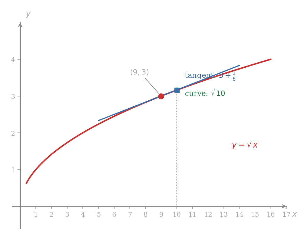
Estimate $\sqrt{10}$ using the tangent line to $y = \sqrt{x}$ at $x = 9$ , and compare with the exact value.

By the power rule, $f'(x) = \tfrac{1}{2}\,x^{-1/2} = 1/(2 \sqrt{x})$ , so at $a = 9$ ,

f(9) = 3, \qquad f'(9) = \tfrac{1}{6}.

The linear approximation supplies

\sqrt{10} = f(10) \approx f(9) + f'(9) = 3 + \tfrac{1}{6} = 3.1\overline{6}.

The exact value is $\sqrt{10} = 3.1623$ to four decimal places, so the approximation overshoots by about $0.005$ . The tangent line, drawn at $(9, 3)$ with slope $\tfrac{1}{6}$ , sits a little above the curve over $[9, 10]$ because $\sqrt{x}$ bends downwards there.

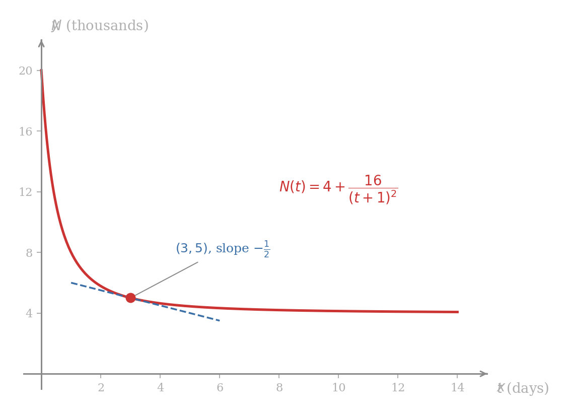
The curve y equals square root of x drawn from x near zero to x equals sixteen, with a tangent line of slope one sixth drawn at the marked point nine comma three. A vertical dotted segment at x equals ten meets two close points, one on the tangent line at height three plus one sixth and one slightly lower on the curve at the height square root of ten, illustrating that the tangent value approximates the curve value with a small overshoot.

Example 20 (Falling sign-ups for a launched product)

A small platform records the number of new sign-ups per day after launch. The empirical fit, valid for the first fortnight, is

N(t) = 4 + \frac{16}{(t + 1)^{2}}, \qquad 0 \leq t \leq 14,

with $t$ measured in days since launch and treated as a continuous variable, and $N$ in thousands of sign-ups per day. Compute $N(3)$ and $N'(3)$ , interpret each, and use the linear approximation to estimate the daily sign-ups on day $4$ .

The height supplies the actual count on day $3$ ,

N(3) = 4 + \frac{16}{16} = 5 \text{ thousand sign-ups}.

The slope is computed by writing the second term as $16\,(t + 1)^{-2}$ and applying the constant multiple rule together with the General power rule with $g(t) = t + 1$ and $r = -2$ ,

N'(t) = 16 \cdot (-2)(t + 1)^{-3} = -\frac{32}{(t + 1)^{3}}.

At $t = 3$ this gives $N'(3) = -32/64 = -\tfrac{1}{2}$ , that is $-500$ sign-ups per day at that instant: the platform is losing half a thousand sign-ups per day from one day to the next. The linear approximation then estimates the day- $4$ count as

N(4) \approx N(3) + N'(3) = 5 - \tfrac{1}{2} = 4.5 \text{ thousand}.

The exact value is $N(4) = 4 + 16/25 = 4.64$ thousand, so the approximation falls short by $0.14$ thousand, or $140$ sign-ups, the discrepancy explained by the bending of $N$ over $[3, 4]$ .

Marginal cost

The publisher of Lesson 2AM had a linear total cost $C(x) = 10{,}000 + 25 x$ , and the marginal cost defined there was the slope $25$ , the additional cost of the next copy at every production level. For a non-linear cost the same reading carries through, but only at one production level at a time, and only as an approximation to the actual additional cost.

Definition 2 (Marginal Cost)

Let $C(x)$ be the total cost of producing $x$ units of a commodity. The marginal cost function is the derivative $C'(x)$ . The marginal cost of producing $a$ units, $C'(a)$ , is by the linear approximation above approximately equal to $C(a + 1) - C(a)$ , the actual additional cost incurred when production is raised by one unit from $a$ to $a + 1$ .

The units of $C'(x)$ follow from the rate-of-change reading: when $C$ is measured in pounds and $x$ is a number of items, $C'(x)$ is measured in pounds per item, the same units the slope of a linear cost function carried in Lesson 2AM. The non-linear definition specialises to the linear one when $C$ is itself linear, in which case $C'(x) = m$ is constant and the approximation becomes exact.

Example 21 (Marginal cost on a non-linear cost function)

A small ceramics studio has total cost

C(x) = 0.004\,x^{3} - 0.6\,x^{2} + 35\,x + 240 \text{ pounds}

for a daily production of $x$ pieces. Compare the actual additional cost of raising production from $40$ to $41$ pieces with the marginal cost at $x = 40$ .

The actual additional cost is $C(41) - C(40)$ , computed directly,

C(40) = 256 - 960 + 1400 + 240 = 936, \qquad C(41) = 275.684 - 1008.6 + 1435 + 240 = 942.084,

so $C(41) - C(40) = 6.084$ pounds. The marginal cost at $x = 40$ is the value of the derivative there, computed by the rules of the previous sections,

C'(x) = 0.012\,x^{2} - 1.2\,x + 35,

giving $C'(40) = 19.2 - 48 + 35 = 6.2$ pounds per piece. The marginal cost $6.2$ approximates the actual increment $6.084$ to within about $0.1$ pound, the residual reflecting the small but non-zero bending of $C$ over $[40, 41]$ .

Marginal revenue and marginal profit

The same construction applies to revenue and profit. If $R(x)$ is the revenue from the sale of $x$ units and $C(x)$ the cost of producing them, the profit is $P(x) = R(x) - C(x)$ . The Sum and Difference Rules give

P'(x) = R'(x) - C'(x),

so marginal profit is marginal revenue minus marginal cost without further work.

Definition 3 (Marginal Revenue, Marginal Profit)

For a revenue function $R(x)$ and a profit function $P(x)$ , the marginal revenue function is $R'(x)$ and the marginal profit function is $P'(x)$ . The marginal revenue of producing $a$ units, $R'(a)$ , approximates $R(a + 1) - R(a)$ , and the marginal profit $P'(a)$ approximates $P(a + 1) - P(a)$ .

The decision whether to raise production by one unit reduces, in linear-approximation terms, to the sign of the marginal profit at the current level: a positive $P'(a)$ predicts that the next unit increases profit, a negative one that it decreases it.

Example 22 (Deciding on a production increase)

A workshop’s revenue from the sale of $x$ tables per week is $R(x)$ thousand pounds, and its cost is

C(x) = 2 + 0.1\,x^{2} \text{ thousand pounds}.

Direct measurement at the current production level $x = 4$ gives $R(4) = 9$ and $R'(4) = -0.6$ thousand pounds per table; the revenue is falling because the workshop is saturating its small local market. Estimate the change in revenue, the change in cost, and the change in profit on raising production to $x = 5$ , and decide whether the increase is worthwhile.

The estimated additional revenue, by the linear approximation, is $R(5) - R(4) \approx R'(4) = -0.6$ thousand pounds, so revenue is predicted to fall by about £600. The marginal cost is $C'(x) = 0.2\,x$ by the rules of the previous sections, giving $C'(4) = 0.8$ thousand pounds per table, and the additional cost is approximately £800. The marginal profit is therefore

P'(4) = R'(4) - C'(4) = -0.6 - 0.8 = -1.4 \text{ thousand pounds per table},

predicting a profit drop of about £1400 if production is raised to $x = 5$ . Despite the workshop running at the level profit $P(4) = R(4) - C(4) = 9 - 3.6 = 5.4$ thousand pounds, the increase is not worthwhile: the next table is forecast to remove £1400 from the weekly profit. Level and rate of change tell different stories, and the marginal calculation reads only the second.

Problem 7

A small bakery’s daily total cost is

C(x) = 0.01\,x^{3} - 0.9\,x^{2} + 30\,x + 80 \text{ pounds}

for a daily production of $x$ loaves. Compute $C'(x)$ by the rules of the previous sections, evaluate the marginal cost at $x = 30$ , and compare with the exact additional cost $C(31) - C(30)$ .

Problem 8

A streaming service’s monthly revenue from the sale of $x$ thousand subscriptions is $R(x)$ million pounds, with $R(20) = 12$ and $R'(20) = 0.4$ million pounds per thousand subscriptions. The corresponding cost is $C(x) = 6 + \tfrac{1}{2} \sqrt{x}$ million pounds.

Estimate $R(21)$ by the linear approximation.
Compute $C(20)$ and $C(21) - C(20)$ exactly, and compare the second with the marginal cost $C'(20)$ .
Compute the marginal profit $P'(20)$ and decide whether raising production to $21$ thousand subscriptions is worthwhile.

Average Rates of Change

The previous section read $f'(a)$ as the rate of change of $f$ at $x = a$ , the slope of the tangent line at $(a, f(a))$ . A second rate of change is sometimes more natural: the average rate of change of $f$ over a whole interval, computed by dividing the total change in the output by the length of the interval. The two readings are linked by the secant construction of Lesson 2PM.

Definition 4 (Average Rate of Change)

The average rate of change of $f(x)$ over an interval $a \leq x \leq b$ with $a < b$ is the ratio

\frac{f(b) - f(a)}{b - a},

the change in $f$ divided by the length of the interval. Geometrically, it is the slope of the secant line through $(a, f(a))$ and $(b, f(b))$ .

When $b = a + h$ the length of the interval is $h$ , the change in $f$ is $f(a + h) - f(a)$ , and the ratio collapses to the difference quotient of Lesson 2PM,

\frac{f(a + h) - f(a)}{h},

the same expression whose limit as $h \to 0$ is $f'(a)$ . Letting the interval shrink to a single point therefore turns the average rate into the instantaneous rate, and the two are one construction read at its two extremes. From this point onwards, unless the qualifier average is used explicitly, the phrase rate of change will mean the instantaneous rate $f'(a)$ .

Example 23 (Average rates approaching the instantaneous rate)

For $f(x) = x^{2}$ , compute the average rate of change of $f$ over each of the intervals $[1, 2]$ , $[1, 1.1]$ , and $[1, 1.01]$ , and compare with the instantaneous rate $f'(1)$ .

The power rule gives $f'(x) = 2 x$ and $f'(1) = 2$ . The three average rates are

\frac{f(2) - f(1)}{2 - 1} = \frac{4 - 1}{1} = 3,

\frac{f(1.1) - f(1)}{1.1 - 1} = \frac{1.21 - 1}{0.1} = 2.1,

\frac{f(1.01) - f(1)}{1.01 - 1} = \frac{1.0201 - 1}{0.01} = 2.01.

The averages drop from $3$ to $2.1$ to $2.01$ as the right endpoint approaches $1$ , in agreement with $f'(1) = 2$ in the limit. The pattern is the secant slopes of Lesson 2PM tending to the tangent slope as the second point slides towards the first.

The parabola y equals x squared drawn near the point one comma one. Three dashed secant lines are drawn from one comma one to the points two comma four, one point one comma one point two one, and one point zero one comma one point zero two zero one, with the second points of each secant marked. A solid black tangent line of slope two passes through one comma one as well, with the secant slopes labelled three, two point one, and two point zero one approaching the tangent slope of two as the second point slides towards the first.

Problem 9

For $f(x) = x^{3}$ , compute the average rate of change over each of the intervals $[2, 3]$ , $[2, 2.1]$ , and $[2, 2.01]$ , then compute $f'(2)$ by the power rule and verify that the averages approach it.

Reading rates from a graph

When $f$ is supplied by a graph rather than a formula, both rates can be read off without any algebra. The average rate over an interval is the slope of the secant line connecting the two endpoints, supplied by slope property 2 of Lesson 2AM. The instantaneous rate at a point is the slope of the tangent line at that point, read either by slope property 1 or, when a second point on the tangent is available, by slope property 2 again.

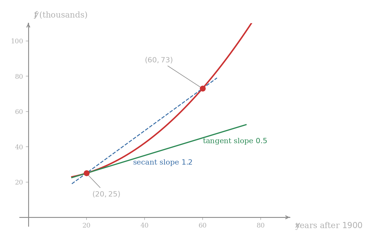
Example 24 (A population model read off a graph)

The function $f(t)$ records the population of a coastal city, in thousands of inhabitants, $t$ years after $1900$ . The graph of $f$ shows

f(20) = 25, \qquad f(60) = 73,

and a tangent line drawn at $(20, 25)$ passes through the further point $(70, 50)$ .

(a) Average rate of growth from $1920$ to $1960$ . By the definition,

\frac{f(60) - f(20)}{60 - 20} = \frac{73 - 25}{40} = 1.2 \text{ thousand inhabitants per year},

so over those forty years the city’s population grew on average at $1{,}200$ inhabitants per year.

(b) Rate of growth in $1920$ . The tangent line at $(20, 25)$ passes through $(70, 50)$ , so by slope property 2 of Lesson 2AM its slope is

f'(20) = \frac{50 - 25}{70 - 20} = 0.5 \text{ thousand inhabitants per year},

that is, in $1920$ the population was growing at $500$ inhabitants per year.

(c) Comparison. The average over $[20, 60]$ , $1{,}200$ per year, exceeds the instantaneous rate at the left endpoint, $500$ per year, indicating that the rate of growth was higher later in the interval than at the start: the curve is steepening as $t$ increases. The average rate is the slope of the secant from $(20, 25)$ to $(60, 73)$ ; the instantaneous rate at $1920$ is the slope of the tangent at $(20, 25)$ alone. The two coincide only when $f$ is linear over the interval.

An increasing population curve drawn against years after 1900, with the two endpoint values twenty comma twenty-five and sixty comma seventy-three marked. A dashed secant line connects the two endpoints with slope one point two thousand inhabitants per year, and a solid tangent line drawn at the leftmost point twenty comma twenty-five has the smaller slope zero point five thousand inhabitants per year, the disparity between the two readings recording that the curve is steepening as t increases.

Problem 10

A graph of fuel remaining against time over a four-hour generator run shows the values

F(0) = 200, \qquad F(2) = 168, \qquad F(4) = 144,

in litres after $t$ hours, and a tangent line drawn at $(2, 168)$ passes through $(4, 142)$ .

Compute the average rate of change of $F$ over the first two hours.
Compute the average rate over the second two hours.
Compute the instantaneous rate of change of $F$ at $t = 2$ .
Order the three numbers and explain what the ordering says about the bending of $F$ .

Velocity, Acceleration, and Estimating Changes

The rate-of-change reading of the derivative covers a family of physical settings in which one quantity is a function of another. Two recurring instances, important enough to fix names for, are the position of a moving object as a function of time, whose rate of change is velocity, and the velocity itself, whose rate of change is acceleration. A second extension, parallel to the marginal-cost discussion two sections back, generalises the one-unit linear approximation to a step of arbitrary length $h$ .

Velocity and acceleration

Suppose an object moves along a straight line, and let $s(t)$ denote its directed position from a fixed reference point at time $t$ , with the convention that one direction along the line is positive and the other negative. Over a short time interval from $t$ to $t + h$ the object’s average velocity is

\frac{s(t + h) - s(t)}{h},

the average rate of change of position over $[t, t + h]$ in the sense of the previous section. Letting $h$ shrink to zero turns the average into an instantaneous velocity at the instant $t$ . Its absolute value is the speed.

Definition 5 (Velocity and Acceleration)

Let $s(t)$ be the position of an object moving along a straight line at time $t$ . The velocity of the object at time $t$ is the derivative $v(t) = s'(t)$ . The acceleration at time $t$ is the derivative of the velocity, $a(t) = v'(t)$ , equivalently the second derivative of the position,

a(t) = s''(t).

A negative velocity records motion in the negative direction along the line, and a negative acceleration records that the velocity is itself decreasing in the chosen sign convention.

The acceleration uses the second derivative of two sections back: differentiating the position once gives the rate at which the position is changing, and differentiating again gives the rate at which that rate is itself changing.

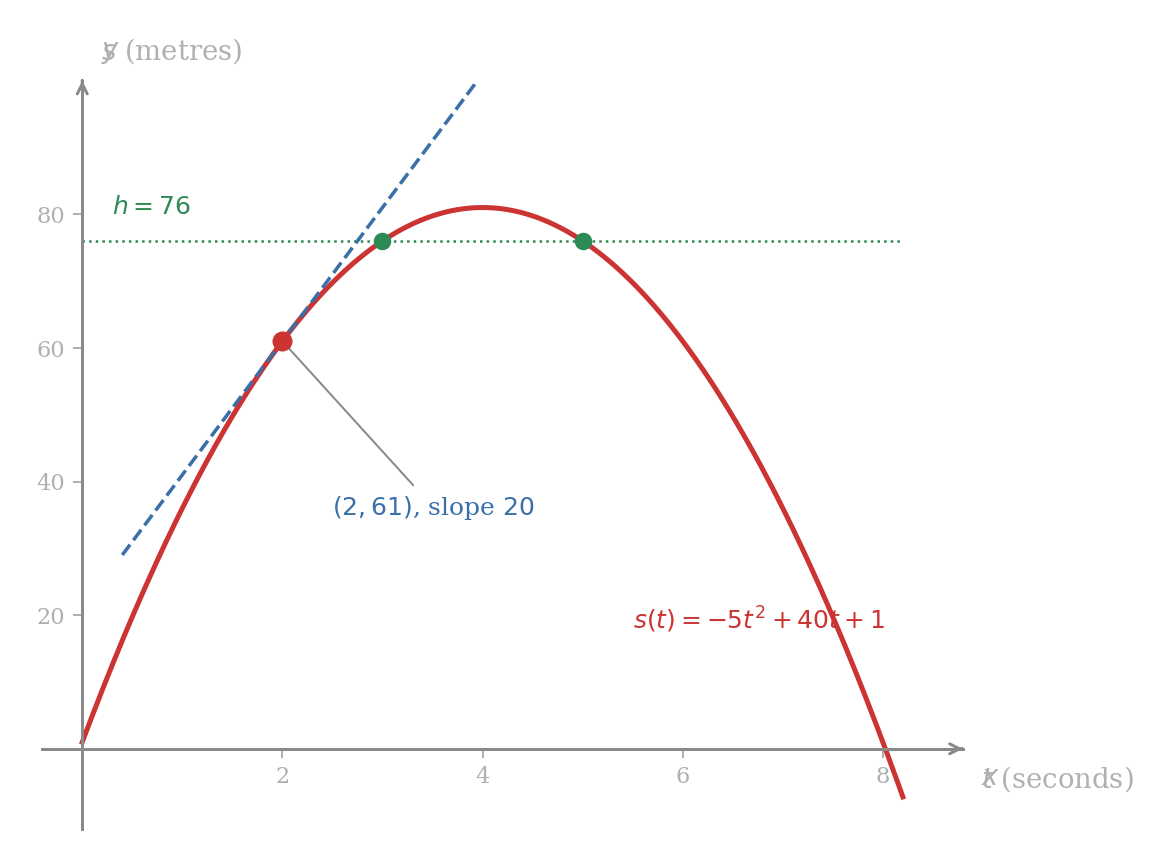
Example 25 (A stone thrown vertically upwards)

A stone is launched vertically upwards from a height of $1$ metre above the ground with an initial velocity of $40$ metres per second. Taking the upward direction as positive and ignoring air resistance, the height after $t$ seconds is

s(t) = -5\,t^{2} + 40\,t + 1 \text{ metres},

the coefficient $-5$ being half the gravitational acceleration of about $10$ metres per second per second.

(a) Velocity at $t = 2$ . The Sum and power rules give $v(t) = s'(t) = -10\,t + 40$ , so $v(2) = 20$ metres per second; the stone is rising at $20$ metres per second two seconds into its flight.

(b) Acceleration at $t = 2$ . Differentiating again, $a(t) = v'(t) = -10$ metres per second per second for every $t$ . The acceleration is negative because gravity acts downwards, the convention having taken upward as positive, and is the same number at every $t$ because the gravitational pull does not vary over the flight.

(c) When is the velocity $-20$ metres per second? Setting $v(t) = -20$ gives $-10\,t + 40 = -20$ , so $t = 6$ seconds. The negative sign records that the stone is now falling at $20$ metres per second.

(d) When is the stone at a height of $76$ metres? Setting $s(t) = 76$ gives

-5\,t^{2} + 40\,t + 1 = 76, \qquad t^{2} - 8\,t + 15 = 0,

which factors as $(t - 3)(t - 5) = 0$ by the inspection of Recitation 1, so $t = 3$ or $t = 5$ . The stone passes through the height $76$ metres twice: once on the way up at $t = 3$ seconds and once on the way down at $t = 5$ seconds.

The downward-opening parabolic position curve s of t equals minus five t squared plus forty t plus one drawn from t equals zero to t equals about eight seconds. A dashed tangent line of slope twenty drawn at the marked point two comma sixty-one captures the velocity at that instant, and a horizontal dotted line at height seventy-six crosses the curve at the marked points three comma seventy-six and five comma seventy-six, recording the two times at which the stone passes through that height.

Problem 11

A bead slides along a straight wire with directed position $s(t) = t^{3} - 6\,t^{2} + 9\,t$ metres at time $t$ seconds, $t \geq 0$ .

Compute the velocity and the acceleration as functions of $t$ .
Find every time at which the bead is momentarily at rest, $v(t) = 0$ .
Find the time at which the acceleration is zero, and state the velocity at that instant.

The change in $f$ over a step of length $h$

The marginal-cost reading two sections back approximated the change in cost across a step of one unit by $C'(a)$ . The same construction extends to a step of arbitrary length, the only modification a multiplication of the rate by the length of the step.

Note (Linear approximation over a step of length $h$)

For $f$ differentiable at $x = a$ and a small displacement $h$ , positive or negative,

f(a + h) - f(a) \approx f'(a) \cdot h, \qquad \text{equivalently,} \qquad f(a + h) \approx f(a) + f'(a) \cdot h.

Setting $h = 1$ recovers the formula of two sections back. The right-hand side is the change in $y$ along the tangent line at $(a, f(a))$ over a horizontal step of $h$ , by slope property 1 of Lesson 2AM scaled by $h$ ; for small $h$ the curve $y = f(x)$ stays close to the tangent line, and the change along the curve is well approximated by the change along the line.

A smooth curve y equals f of x drawn alongside its tangent line at the marked point a comma f of a. A horizontal step of length h is shown along the x-axis from a to a plus h. Two vertical double-headed arrows on the right show the actual change f of a plus h minus f of a along the curve in one colour, and the linear approximation f prime of a times h along the tangent line in a contrasting colour, with the two endpoints marked separately to make the small discrepancy between the curve value and the tangent value visible.

The same identity may be derived from the equation of the tangent line at $x = a$ written out in Lesson 2PM,

y - f(a) = f'(a)\,(x - a).

Replacing the tangent value $y$ by the curve value $f(x)$ , valid only as an approximation, and substituting $x = a + h$ produces $f(a + h) - f(a) \approx f'(a) \cdot h$ , the same formula obtained directly.

Example 26 (A textile mill's production function)

A textile mill’s daily output is $q(L)$ garments when $L$ person-hours of labour are employed. Direct measurement at the current level $L = 800$ gives

q(800) = 240, \qquad q'(800) = 0.6,

the slope $0.6$ measured in garments per person-hour. Interpret each value, and use the linear approximation to estimate the daily output at $L = 801$ , at $L = 800.25$ , and at $L = 799$ .

The height $q(800) = 240$ records that $800$ person-hours of labour currently produce $240$ garments per day. The slope $q'(800) = 0.6$ records that, at the current level, output rises at the rate of $0.6$ garments for each additional person-hour of labour.

For $L = 801$ the displacement is $h = 1$ , and the linear approximation gives $q(801) \approx 240 + 0.6 = 240.6$ garments. For $L = 800.25$ the displacement is $h = 0.25$ , and

q(800.25) \approx q(800) + q'(800) \cdot 0.25 = 240 + 0.15 = 240.15 \text{ garments}.

For $L = 799$ the displacement is $h = -1$ , and the same formula gives

q(799) \approx q(800) + q'(800) \cdot (-1) = 240 - 0.6 = 239.4 \text{ garments},

so reducing labour by one person-hour drops daily output by about $0.6$ garments. The negative displacement is handled by the formula without further work.

Marginal cost over a non-unit step

Specialising the new approximation to a cost function $C(x)$ with displacement $h$ ,

C(a + h) - C(a) \approx C'(a) \cdot h.

For $h = 1$ this collapses to the marginal-cost formula of two sections back; for $h \neq 1$ the marginal cost is scaled in proportion to the length of the step.

Example 27 (Marginal cost on a quadratic cost function)

A workshop’s total cost of producing $x$ units of a commodity is

C(x) = 4\,x^{2} + 5\,x + 20 \text{ thousand pounds}.

Find the marginal cost function, evaluate the cost and the marginal cost at the production level $x = 8$ , estimate the cost of the ninth unit, and estimate the additional cost of raising production from $8$ to $8.5$ units.

The Sum, Constant-Multiple, and power rules give $C'(x) = 8\,x + 5$ , the marginal cost function in thousand pounds per unit. At $x = 8$ ,

C(8) = 256 + 40 + 20 = 316, \qquad C'(8) = 64 + 5 = 69.

The cost of the ninth unit is $C(9) - C(8)$ , and by the marginal approximation with $h = 1$ this is approximately $C'(8) = 69$ thousand pounds. The additional cost of raising production from $8$ to $8.5$ has step $h = 0.5$ , so the same formula gives

C(8.5) - C(8) \approx C'(8) \cdot 0.5 = 69 \cdot 0.5 = 34.5 \text{ thousand pounds}.

Halving the step size halves the predicted change in cost, a feature the unit-step formula of two sections back was unable to express.

Units of a rate of change

The rate-of-change reading fixes the units of $f'(x)$ from those of $f(x)$ and $x$ . Because $f'(x)$ is computed as a change in $f$ divided by a change in $x$ , the units of $f'(x)$ are

\text{units of } f'(x) = \frac{\text{units of } f(x)}{\text{units of } x}.

The examples in this lesson supply several instances at once: position in metres against time in seconds gives velocity in metres per second; velocity in metres per second against time in seconds gives acceleration in metres per second per second; cost in pounds against units of production gives marginal cost in pounds per unit; output in garments against person-hours of labour gives marginal product in garments per person-hour. Stating the units alongside the numerical answer is part of the answer in any rate-of-change calculation.

Exercises

Exercise 1

Differentiate $f(x) = 5 x^{4} - 2 x^{3} + 7 x - 11$ by the rules of this section, and evaluate $f'(1)$ .

Exercise 2

Find the equation of the tangent line to $y = 2 x^{3} - x + 4$ at $x = -1$ , in slope-intercept form.

Exercise 3

Show that the curve $y = x^{4} - 2 x^{2} + 3$ has exactly three horizontal tangents, and locate each of them.

Exercise 4

Differentiate $f(x) = (5 x - 2)^{6}$ by the General power rule, and confirm the answer at $x = 1$ by expanding $(5 x - 2)^{6}$ to a polynomial in $x$ and differentiating term by term.

Exercise 5

Differentiate $f(x) = \sqrt{x^{2} + 9}$ , state the natural domain of $f'$ , and write the equation of the tangent line at the point $(4, 5)$ .

Exercise 6

For $f(x) = (1 + 2 x)^{-2}$ on $x \neq -\tfrac{1}{2}$ , compute $f'(x)$ by the General power rule, then verify by writing $f(x) = 1 / (1 + 2 x)^{2}$ and applying the General power rule with $r = -2$ instead.

Exercise 7

Differentiate $f(r) = \pi r^{2}$ with respect to $r$ , treating $\pi$ as a constant by the constant multiple rule. Recognising $f(r)$ as the area of a disc of radius $r$ , identify the geometric quantity the derivative equals.

Exercise 8

Compute $\dfrac{d}{dz}\bigl((z^{2} - 6 z + 9)^{5}\bigr)$ by the General power rule, and verify the answer by first writing $z^{2} - 6 z + 9 = (z - 3)^{2}$ and so $(z^{2} - 6 z + 9)^{5} = (z - 3)^{10}$ , then differentiating the rewritten form.

Exercise 9

For $y = x^{4} - 3 x^{2} + 7$ , compute

\left.\frac{d}{dx}\!\left(\frac{dy}{dx}\right)\right|_{x = 2}

by differentiating twice and substituting.

Exercise 10

After a publicity drive ends, the daily downloads of a mobile app, in thousands, are modelled by

D(t) = -2\,t^{2} + 24\,t + 80, \qquad 0 \leq t \leq 12,

days from the end of the drive. Compute the average rate of change of $D$ over the interval $[3, 4]$ , and the instantaneous rate of change at $t = 2$ .

Exercise 11

Let $f(p)$ denote the number, in thousands, of headphones sold per month when the price is set at $\pounds p$ per pair. Suppose

f(80) = 12 \qquad \text{and} \qquad f'(80) = -0.5.

Interpret each value, then estimate the monthly sales when the price is raised to $\pounds 85$ per pair.

Exercise 12

Let $P(x)$ denote the profit, in pounds, from manufacturing and selling $x$ specialty bicycles per month. Suppose

P(50) = 45{,}000 \qquad \text{and} \qquad P'(50) = 800.

Interpret each value, and use the linear approximation to estimate the profit from manufacturing and selling $49$ bicycles per month.