Lesson 4PM: Implicit Differentiation and Related Rates

04/03/2026

#Math#Differentiation

← Back to MA0A: Differentiation

Video

Lesson assets

video link

CS50P Lecture 0: Functions, Variables

recitation

Recitation

Homework 4 PDF

Lesson 4AM closed with the chain rule and a small toolkit for time rates of change: pick an inner variable that depends on $t$ , an outer quantity that depends on the inner variable, and multiply the two derivatives. Every example there shared a structural feature — the relationship between the variables was given by an honest function, $V = \frac{4}{3} \pi r^3$ , $R = -0{.}002 \, x^2 + 86 \, x$ , and so on. The slope formula came out of differentiating that function once.

Plenty of curves in geometry and economics are not given as a function. The circle $x^2 + y^2 = 4$ assigns two values of $y$ to most $x$ in $(-2, 2)$ , and so fails the vertical-line test from Lesson 1AM. The production isoquant $60 \, x^{3/4} y^{1/4} = 3240$ that an economist scrawls on a board is a curve in the plane, but solving for $y$ algebraically is rarely what one wants to do. These equations implicitly define a relationship; the question is whether the slope of that relationship can be read off without first untangling $y$ from $x$ .

The chain rule (already in hand) handles the job, and it lets us answer two different questions about the same equation. Treating $y$ as an unknown function $y = g(x)$ and differentiating with respect to $x$ produces a linear equation in $\frac{dy}{dx}$ , solvable by ordinary algebra. Treating both $x$ and $y$ as unknown functions of a third variable $t$ (typically time) and differentiating with respect to $t$ produces a linear equation in $\frac{dx}{dt}$ and $\frac{dy}{dt}$ , expressing the related rates of two quantities tied together by the curve. The first half of this lesson develops the static slope picture; the second half upgrades it to motion.

Curves That Aren’t Function Graphs

Consider the circle

x^2 + y^2 = 4. \tag{1}

Its graph (Fig. 1) is the set of points two units from the origin. Because there are two points with $x$ -coordinate $1$ , namely $(1, \sqrt{3})$ and $(1, -\sqrt{3})$ , the relation is not the graph of any function $y = f(x)$ .

Locally, however, it behaves like one. Stay near $(1, \sqrt{3})$ : the upper half of the circle close to that point is the graph of $y = \sqrt{4 - x^2}$ , a perfectly good function on $(-2, 2)$ . Stay near $(1, -\sqrt{3})$ and the relevant local function is $y = -\sqrt{4 - x^2}$ . Wherever the tangent line is not vertical, the curve looks like a function graph in a small enough neighborhood, and the slope of the curve at $(a, b)$ is the slope of that local function at $x = a$ . Standard notation isolates the point at which the slope is read:

\left. \frac{dy}{dx} \right|_{\substack{x = a\\ y = b}}.

Both coordinates appear because, on a curve like the circle, the slope at $x = 1$ is ambiguous until we say which of $(1, \sqrt{3})$ or $(1, -\sqrt{3})$ we mean.

Definition 35 (Implicit function)

An equation $F(x, y) = 0$ is said to define $y$ implicitly as a function of $x$ near a point $(a, b)$ on the curve $F(x, y) = 0$ if there is a function $g$ , defined on an open interval around $a$ , such that $g(a) = b$ and $F(x, g(x)) = 0$ for every $x$ in that interval. The slope $\frac{dy}{dx}\big|_{(a, b)}$ is the derivative $g'(a)$ .

Circle x² + y² = 4 with the points (1, √3) and (1, -√3) marked. Tangent lines drawn at each point, with the upper tangent sloping at -1/√3 and the lower tangent sloping at +1/√3.

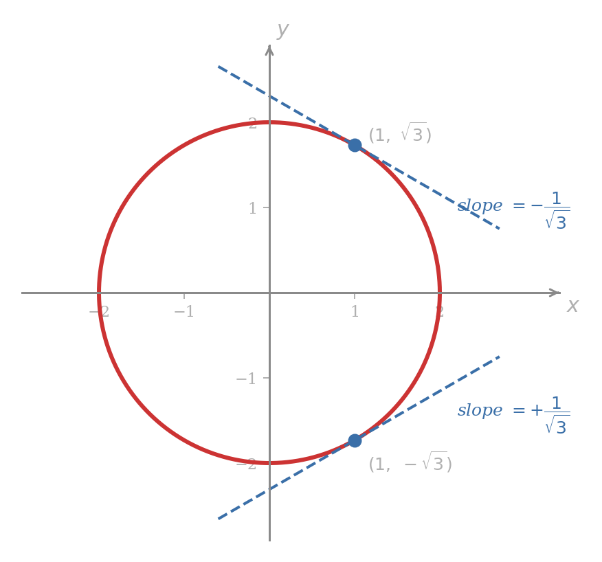
The figure shows the two tangent slopes that this lesson is about to compute. Throughout, we assume the equation in question implicitly defines a differentiable function near every point we sample; the points where this fails (the leftmost and rightmost points of the circle, where the tangent is vertical) appear as the points at which the slope formula divides by zero.

The Implicit Differentiation Move

Treat $y$ as an unspecified differentiable function of $x$ , write $y = g(x)$ in your head, and apply the chain rule whenever a power or composition of $y$ is differentiated. Every other rule from the toolkit table at the end of Lesson 4AM applies as before.

The single new pattern is this: differentiating $y^r$ with respect to $x$ is not the same as differentiating it with respect to $y$ . The general power rule, with $g(x)$ playing the role of the inner function, gives

\frac{d}{dx}\bigl[ g(x) \bigr]^r = r \, [g(x)]^{r-1} \, g'(x).

Substituting $y = g(x)$ and $g'(x) = \frac{dy}{dx}$ yields the working form.

Theorem 16 (Differentiating a power of

y

with respect to

x

)

If $y$ is a differentiable function of $x$ and $r$ is a constant for which $y^{r-1}$ makes sense at the point in question, then

\frac{d}{dx} y^r = r \, y^{r-1} \, \frac{dy}{dx}. \tag{2}

Proof

Set $g(x) = y$ and $f(u) = u^r$ . The composition $f(g(x)) = y^r$ is differentiated by the chain rule of Lesson 4AM:

\frac{d}{dx} y^r = f'(g(x)) \cdot g'(x) = r [g(x)]^{r-1} \cdot g'(x) = r \, y^{r-1} \, \frac{dy}{dx}.

The last equality only restates $g(x) = y$ and $g'(x) = \frac{dy}{dx}$ .

■

The factor $\frac{dy}{dx}$ is the bookkeeping that distinguishes a $y$ -power from an $x$ -power: an $x$ -power gets no such factor because $\frac{dx}{dx} = 1$ . Forgetting it is the single most common error, and every implicit differentiation in the rest of this lesson contains at least one application of $(2)$ .

A First Slope: The Circle

Example 123 (Tangent slopes on the radius-2 circle)

Use implicit differentiation to find $\dfrac{dy}{dx}$ for the circle $x^2 + y^2 = 4$ from $(1)$ . Then evaluate the slope at the points $(1, \sqrt{3})$ and $(1, -\sqrt{3})$ .

Differentiate both sides of $x^2 + y^2 = 4$ with respect to $x$ . The left side splits by the sum rule. The first piece $x^2$ has derivative $2 x$ as usual. The second piece $y^2$ is a power of $y$ , so by $(2)$ ,

\frac{d}{dx} y^2 = 2 y \, \frac{dy}{dx}.

The right side, the constant $4$ , has derivative $0$ . Thus

2 x + 2 y \, \frac{dy}{dx} = 0.

Solving for $\frac{dy}{dx}$ when $y \neq 0$ ,

2 y \, \frac{dy}{dx} = -2 x.

Dividing both sides by $2y$ gives

\frac{dy}{dx} = -\frac{x}{y}. \tag{3}

Equation $(3)$ depends on both coordinates, which is exactly right: the slope at $x = 1$ is genuinely two-valued on the circle, and the formula resolves the ambiguity by asking for $y$ as well.

At $(1, \sqrt{3})$ :

\left. \frac{dy}{dx} \right|_{\substack{x = 1\\ y = \sqrt{3}}} = -\frac{1}{\sqrt{3}}.

At $(1, -\sqrt{3})$ :

\left. \frac{dy}{dx} \right|_{\substack{x = 1\\ y = -\sqrt{3}}} = -\frac{1}{-\sqrt{3}} = \frac{1}{\sqrt{3}}.

The two slopes are negatives of each other; geometrically, the upper and lower tangents reflect across the $x$ -axis, and their slopes flip sign. The slope formula $(3)$ fails at the points $(\pm 2, 0)$ because the denominator $y$ vanishes there; those are precisely the two points at which the tangent is vertical and the slope is undefined.

The same answer is obtained, with more work, by solving $(1)$ for $y$ on each half of the circle and differentiating the explicit formula. On the upper half $y = \sqrt{4 - x^2}$ , the chain rule gives

\frac{dy}{dx} = \frac{-x}{\sqrt{4 - x^2}} = -\frac{x}{y}.

The implicit answer $-x/y$ contains both halves at once. Two cases collapse into one expression — that is the structural payoff.

Example 124 (A tangent line from the implicit slope)

Find the tangent line to the circle

x^2+y^2=4

at the point $(1,\sqrt{3})$ .

The slope formula from $(3)$ gives

\left.\frac{dy}{dx}\right|_{\substack{x=1\\ y=\sqrt{3}}}=-\frac{1}{\sqrt{3}}.

The tangent line is the line through $(1,\sqrt{3})$ with this slope, so the point-slope form is

y-\sqrt{3}=-\frac{1}{\sqrt{3}}(x-1).

If desired, multiply through by $\sqrt{3}$ to remove the fraction:

\sqrt{3}\,y-3=-(x-1),

or equivalently

x+\sqrt{3}\,y=4.

The final form has a geometric reading: the radius from the origin to $(1,\sqrt{3})$ has slope $\sqrt{3}$ , while the tangent slope is $-1/\sqrt{3}$ , so the radius and tangent are perpendicular.

Problem 127

For the ellipse $\dfrac{x^2}{9} + \dfrac{y^2}{4} = 1$ :

Use implicit differentiation to find $\dfrac{dy}{dx}$ .
Compute the slopes of the tangent lines at $\left(\tfrac{3}{2}, \sqrt{3}\right)$ and $\left(\tfrac{3}{2}, -\sqrt{3}\right)$ . Confirm they are negatives of each other and explain why geometrically.
Locate the points at which the tangent is horizontal and the points at which it is vertical, by reading off when the numerator and denominator of $\dfrac{dy}{dx}$ vanish.

Products, Sums, and Mixed Terms

Two short examples cover the rest of the technique. Whenever $y$ multiplies $x$ , the product rule applies; whenever $y$ is raised to a power, $(2)$ applies; and the two combine without surprises.

Example 125 (A two-factor implicit equation)

Use implicit differentiation to compute $\dfrac{dy}{dx}$ for $x^2 y^6 = 1$ .

Differentiate each side with respect to $x$ . The left side is a product, so the product rule supplies

x^2 \cdot \frac{d}{dx} (y^6) + y^6 \cdot \frac{d}{dx} (x^2) = \frac{d}{dx}(1).

The first $\frac{d}{dx}$ is a power of $y$ , evaluated by $(2)$ with $r = 6$ , giving $6 y^5 \, \frac{dy}{dx}$ . The second is the ordinary power rule, giving $2 x$ . The right side has derivative $0$ . Combining,

6 \, x^2 y^5 \, \frac{dy}{dx} + 2 x \, y^6 = 0.

Move the term without $\frac{dy}{dx}$ to the right and divide by the coefficient of $\frac{dy}{dx}$ :

6 \, x^2 y^5 \, \frac{dy}{dx} = -2 x \, y^6.

Dividing both sides by $6x^2y^5$ and simplifying,

\frac{dy}{dx} = -\frac{2 x \, y^6}{6 \, x^2 y^5} = -\frac{y}{3 x}.

Provided $x \neq 0$ and $y \neq 0$ — both forced by the original constraint $x^2 y^6 = 1$ — the slope is given by a tidy ratio. No part of the calculation required isolating $y$ as a function of $x$ .

Example 126 (A four-term mixture)

Use implicit differentiation to find $\dfrac{dy}{dx}$ when $x^2 y + x y^3 - 3 x = 5$ .

Differentiate term by term. Both $x^2 y$ and $x y^3$ are products and need the product rule. The term $-3 x$ contributes $-3$ , and the constant $5$ contributes $0$ :

\underbrace{x^2 \cdot \frac{dy}{dx} + y \cdot 2 x}_{\text{from } x^2 y} + \underbrace{x \cdot 3 y^2 \frac{dy}{dx} + y^3 \cdot 1}_{\text{from } x y^3} - 3 = 0.

That is the entire calculus content of the calculation. What remains is algebra: collect $\frac{dy}{dx}$ on the left, send everything else to the right, and divide.

Step 1 — keep the $\frac{dy}{dx}$ terms together:

x^2 \frac{dy}{dx} + 3 x y^2 \frac{dy}{dx} = 3 - y^3 - 2 x y.

Step 2 — factor out $\frac{dy}{dx}$ :

(x^2 + 3 x y^2) \frac{dy}{dx} = 3 - y^3 - 2 x y.

Step 3 — divide by the coefficient:

\frac{dy}{dx} = \frac{3 - y^3 - 2 x y}{x^2 + 3 x y^2}.

The answer mixes $x$ and $y$ , just as $(3)$ did for the circle. The original equation does not factor; the slope formula is forced to depend on both coordinates because the curve does.

Note (The procedure)

Three of these calculations are enough to pull out the procedure that runs them all.

Differentiate every term of the equation with respect to $x$ . Use the product rule for any term that contains both $x$ and $y$ as factors. Use $(2)$ for any pure power of $y$ .
Move every term containing $\frac{dy}{dx}$ to one side and every term without it to the other.
Factor $\frac{dy}{dx}$ out of the side it lives on.
Divide by the factor that multiplies $\frac{dy}{dx}$ .

The end product is a formula for $\frac{dy}{dx}$ in terms of $x$ and $y$ . To evaluate the slope at a specific point, substitute both coordinates of that point.

Problem 128

Find $\dfrac{dy}{dx}$ for each curve and state the points (if any) at which the formula breaks down.

$x^3 + y^3 = 9$ .
$x y^2 - x^2 y = 6$ .
$\sqrt{x} + \sqrt{y} = 4$ .
$x^2 - 2 x y + 3 y^2 = 8$ .

Problem 129

The curve $y^2 = x^3 - 3 x + 3$ is an elliptic curve (a class central to modern number theory and cryptography).

Use implicit differentiation to express $\dfrac{dy}{dx}$ in terms of $x$ and $y$ .
The point $(1, 1)$ lies on the curve. Find the equation of the tangent line at $(1, 1)$ .
Find every point on the curve at which the tangent is horizontal.

Problem 130

Two curves are orthogonal at a point of intersection if their tangent lines there are perpendicular — equivalently, if the product of their slopes is $-1$ . Show that the family of circles $x^2 + y^2 = c^2$ ( $c > 0$ ) and the family of lines $y = m x$ ( $m \neq 0$ ) are orthogonal at every point where they cross. Use implicit differentiation on the circle and explicit differentiation on the line.

Problem 131

Consider the curve

y^{3} + y = x^{2}. \tag{$\star$}

Show that for every real $x$ , equation $(\star)$ has exactly one real solution $y$ . (Hint: the function $\varphi(y) = y^{3} + y$ is strictly increasing for every real $y$ — verify with its derivative — and takes every real value, so it is invertible.) Conclude that $(\star)$ defines $y$ implicitly as a function of $x$ at every real $x$ .
Use implicit differentiation to find $\dfrac{dy}{dx}$ in terms of $x$ and $y$ .
Show that $\dfrac{dy}{dx} > 0$ for $x > 0$ and $\dfrac{dy}{dx} < 0$ for $x < 0$ , and identify the unique point on the curve at which $\dfrac{dy}{dx} = 0$ . Tie the sign-change picture to the symmetry $x \mapsto -x$ of equation $(\star)$ .

Production Isoquants and the Marginal Rate of Substitution

Two production inputs — labor $x$ and capital $y$ , say — combine through a Cobb–Douglas technology to produce a fixed level of output. Holding the output constant traces out a curve in the $(x, y)$ -plane called an isoquant: every $(x, y)$ on the curve produces the same total. The slope of the isoquant tells the firm how much of one input must be sacrificed to gain one extra unit of the other while keeping output unchanged.

Example 127 (Isoquant slope and the marginal rate of substitution)

A production process satisfies

60 \, x^{3/4} y^{1/4} = 3240, \tag{4}

where $x$ and $y$ are the amounts of two basic inputs and $3240$ is the fixed output level. Find the slope of the isoquant at the point $(81, 16)$ , and interpret the answer economically.

Differentiate $(4)$ with respect to $x$ . The left side is a product of $60 \, x^{3/4}$ and $y^{1/4}$ , so the product rule gives

60 \, x^{3/4} \cdot \frac{d}{dx}(y^{1/4}) + y^{1/4} \cdot \frac{d}{dx}(60 \, x^{3/4}) = 0.

The two derivatives:

\frac{d}{dx}(y^{1/4}) = \frac{1}{4} y^{-3/4} \, \frac{dy}{dx}, \qquad \frac{d}{dx}(60 \, x^{3/4}) = 60 \cdot \frac{3}{4} x^{-1/4} = 45 \, x^{-1/4}.

Substituting,

60 \, x^{3/4} \cdot \frac{1}{4} y^{-3/4} \frac{dy}{dx} + y^{1/4} \cdot 45 \, x^{-1/4} = 0,

which tidies to

15 \, x^{3/4} y^{-3/4} \, \frac{dy}{dx} = -45 \, x^{-1/4} y^{1/4}.

Dividing,

\frac{dy}{dx} = \frac{-45 \, x^{-1/4} y^{1/4}}{15 \, x^{3/4} y^{-3/4}} = -3 \, x^{-1} y = -\frac{3 \, y}{x}. \tag{5}

Plugging in $(81, 16)$ :

\left. \frac{dy}{dx} \right|_{\substack{x = 81\\ y = 16}} = -\frac{3 \cdot 16}{81} = -\frac{16}{27} \approx -0{.}593.

The economic reading is direct. Increasing input $x$ by one unit while staying on the isoquant requires decreasing input $y$ by approximately $\tfrac{16}{27}$ unit, since the slope is negative. The absolute value $|dy/dx| = \tfrac{16}{27}$ is the marginal rate of substitution of the first input for the second. It depends on the current mix $(x, y)$ : at higher levels of $y$ relative to $x$ , the curve is steeper and a small extra unit of $x$ frees up more $y$ .

Production isoquant 60 x^(3/4) y^(1/4) = 3240 plotted as y against x. The curve falls steeply for small x and flattens as x grows. The point (81, 16) is marked with the tangent line of slope -16/27.

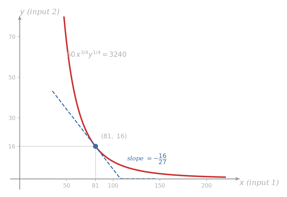
The curve slopes down everywhere — increasing one input lets you reduce the other — and is convex toward the origin. Convexity has a direct economic translation: replacing each unit of input $y$ requires more and more of input $x$ as $y$ becomes scarce, exactly the diminishing-returns behavior the Cobb–Douglas exponent split $3/4 + 1/4 = 1$ is designed to capture. The slope formula $(5)$ encodes this. As $y$ falls and $x$ rises along the isoquant, the ratio $3y/x$ shrinks, so $|dy/dx|$ shrinks — each additional unit of $x$ buys back less and less of $y$ .

Problem 132

A bakery’s daily output (in dozens) of bread depends on flour $x$ (in kilograms) and oven-hours $y$ via the Cobb–Douglas relation

20 \, x^{1/2} y^{1/2} = 360.

Use implicit differentiation to find $\dfrac{dy}{dx}$ as a function of $x$ and $y$ .
Compute the marginal rate of substitution at $(x, y) = (16, 81)$ and interpret in plain English.
Confirm part (1) by solving the equation explicitly for $y$ and differentiating, and check that the two answers agree on the curve.

Problem 133

A consumer’s preferences are summarized by the indifference curve

x^{2} y = 50, \qquad x, y > 0,

where $x$ is the quantity of one good and $y$ is the quantity of another. Use implicit differentiation to compute $\dfrac{dy}{dx}$ and find the marginal rate of substitution at the bundle $(5, 2)$ . State, in plain English, what the answer says about the consumer’s willingness to swap goods.

A Curve from the 17th Century

Implicit differentiation is older than the limit-based theory of derivatives. Descartes communicated the curve below to Fermat in 1638, asking for its tangent at a non-trivial point, and the answer is a single line of implicit differentiation today.

Example 128 (Folium of Descartes)

The folium of Descartes is the curve

x^3 + y^3 = 3 \, x \, y. \tag{6}

Find $\dfrac{dy}{dx}$ in terms of $x$ and $y$ , and use it to determine the slope at the point $\left(\tfrac{3}{2}, \tfrac{3}{2}\right)$ .

Differentiate $(6)$ with respect to $x$ . The left side is a sum, so each term yields its own derivative; $y^3$ uses $(2)$ . The right side $3 x y$ is a product:

3 x^2 + 3 y^2 \frac{dy}{dx} = 3 \! \left(x \cdot \frac{dy}{dx} + y \cdot 1\right).

Cancel the common factor $3$ :

x^2 + y^2 \frac{dy}{dx} = x \, \frac{dy}{dx} + y.

Move $\frac{dy}{dx}$ terms to one side:

y^2 \frac{dy}{dx} - x \, \frac{dy}{dx} = y - x^2.

Factoring out $\frac{dy}{dx}$ gives

(y^2 - x) \frac{dy}{dx} = y - x^2.

Therefore

\frac{dy}{dx} = \frac{y - x^2}{y^2 - x}. \tag{7}

At $\left(\tfrac{3}{2}, \tfrac{3}{2}\right)$ :

\frac{dy}{dx} = \frac{\tfrac{3}{2} - \tfrac{9}{4}}{\tfrac{9}{4} - \tfrac{3}{2}} = \frac{-\tfrac{3}{4}}{\tfrac{3}{4}} = -1.

The tangent at $\left(\tfrac{3}{2}, \tfrac{3}{2}\right)$ has slope $-1$ , which agrees with the symmetry of the curve under the swap $(x, y) \leftrightarrow (y, x)$ : the line $y = x$ is an axis of symmetry, and the tangent at any point on that axis must be perpendicular to it, hence slope $-1$ .

Folium of Descartes x³ + y³ = 3xy. A loop sits in the first quadrant; two wings extend into the second and fourth quadrants and approach the line y = -x - 1 asymptotically. The point (3/2, 3/2) is marked at the tip of the loop with a tangent line of slope -1.

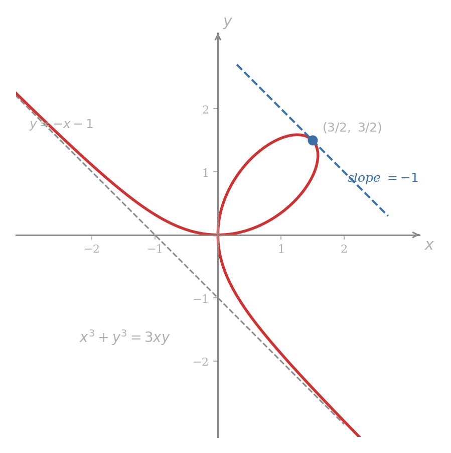
Two structural features of the folium are visible in the picture and explained by $(7)$ . The numerator $y - x^2$ vanishes when $y = x^2$ , giving horizontal tangents; the denominator $y^2 - x$ vanishes when $x = y^2$ , giving vertical tangents. The point $(0, 0)$ is special — both vanish at once, so $(7)$ degenerates to $0/0$ there and the curve has two distinct tangent directions through the origin (visible in the figure as the curve crossing itself).

Problem 134

For the folium $x^3 + y^3 = 3 x y$ :

Find every nonsingular point on the curve at which the tangent is horizontal. Combine the equations $y = x^2$ (numerator zero) and $x^3 + y^3 = 3 x y$ , excluding the origin for now.
Find every nonsingular point at which the tangent is vertical, by combining $x = y^2$ with the curve equation, again excluding the origin for now.
The point $(0, 0)$ is on the curve. Substitute $y = m x$ to find the non-vertical tangent direction at the origin, then use symmetry or substitute $x = n y$ to find the vertical tangent direction. State the two tangent lines.

Problem 135

The lemniscate of Bernoulli is the curve

2 (x^2 + y^2)^2 = 25 (x^2 - y^2).

Use implicit differentiation to find $\dfrac{dy}{dx}$ .
The point $(3, 1)$ lies on the lemniscate (verify). Find the slope of the tangent line at $(3, 1)$ and write the equation of that tangent in point-slope form.

Problem 136

The circle $x^{2} + y^{2} = 4$ and the parabola $y = x^{2} - 2$ intersect at the points $\bigl(\pm\sqrt{3},\, 1\bigr)$ — verify by substituting.

Use implicit differentiation on the circle and the power rule on the parabola to find both tangent slopes at $\bigl(\sqrt{3},\, 1\bigr)$ .
Two curves are orthogonal at a common point if their tangent slopes $m_{1}, m_{2}$ there satisfy $m_{1} m_{2} = -1$ . Decide whether the circle and the parabola meet orthogonally at $\bigl(\sqrt{3},\, 1\bigr)$ .
Without further computation, state the corresponding result at $\bigl(-\sqrt{3},\, 1\bigr)$ , citing the symmetry $x \mapsto -x$ shared by both curves.

In the work so far, $y$ has been a function of $x$ . In many applications the natural independent variable is neither — it is time. A point traces an ellipse as $t$ advances; a market drifts along a demand curve as the price slowly slips; a chemical reaction moves a system along a constraint surface in concentration space. In each case, $x$ and $y$ are both functions of $t$ , neither is given by a formula, and the only relation we have is an equation in $x$ and $y$ that holds at every instant.

The same chain rule that powered implicit differentiation handles this. Differentiating an equation $F(x, y) = c$ with respect to $t$ , and treating $x$ and $y$ as unknown functions $x(t)$ and $y(t)$ , produces a linear equation in the two rates $\dfrac{dx}{dt}$ and $\dfrac{dy}{dt}$ . The equation says nothing about the size of either rate on its own — both can be large or small — but it constrains how they relate. Hence the name: $\dfrac{dx}{dt}$ and $\dfrac{dy}{dt}$ are related rates.

The single bookkeeping change from earlier in the lesson is what plays the role of $\dfrac{dy}{dx}$ in $(2)$ . Now that the independent variable is $t$ , the chain rule applied to $x^r$ and $y^r$ gives

\frac{d}{dt} x^r = r \, x^{r-1} \, \frac{dx}{dt}, \qquad \frac{d}{dt} y^r = r \, y^{r-1} \, \frac{dy}{dt},

and the product rule applied to $x \, y$ gives

\frac{d}{dt}(x \, y) = x \, \frac{dy}{dt} + y \, \frac{dx}{dt}.

Both $x$ and $y$ now generate their own derivative factor, because both depend on $t$ .

Example 129 (A point moving along an ellipse)

The variables $x$ and $y$ are both differentiable functions of $t$ that satisfy

x^2 + 5 \, y^2 = 36 \tag{8}

at every instant.

Differentiate $(8)$ with respect to $t$ and solve for $\dfrac{dy}{dt}$ .
Evaluate $\dfrac{dy}{dt}$ at the moment when $x = 4$ , $y = 2$ , and $\dfrac{dx}{dt} = 5$ .
Differentiating each term of $(8)$ with respect to $t$ , the chain rule supplies one factor of $\dfrac{dx}{dt}$ for the $x^2$ term and one factor of $\dfrac{dy}{dt}$ for the $5 \, y^2$ term:

\frac{d}{dt}(x^2) + \frac{d}{dt}(5 \, y^2) = \frac{d}{dt}(36),

2 x \, \frac{dx}{dt} + 10 \, y \, \frac{dy}{dt} = 0.

Solving for $\dfrac{dy}{dt}$ (whenever $y \neq 0$ ),

\frac{dy}{dt} = -\frac{x}{5 \, y} \, \frac{dx}{dt}. \tag{9}

Substituting $x = 4$ , $y = 2$ , and $\dfrac{dx}{dt} = 5$ :

\frac{dy}{dt} = -\frac{4}{5 \cdot 2} \cdot 5 = -2.

At this instant, the point is moving so that its $y$ -coordinate is decreasing at $2$ units per unit time while the $x$ -coordinate is increasing at $5$ units per unit time. The signs encode direction along the curve.

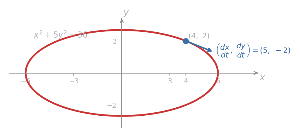
Ellipse x² + 5y² = 36 with semi-axes 6 along x and 6/√5 along y. The point (4, 2) is marked, with a velocity arrow pointing down and to the right showing dx/dt = 5, dy/dt = -2.

The figure shows the ellipse with the velocity vector at $(4, 2)$ . The vector points down-and-right because the point is in the upper half and moving clockwise; the slope of the velocity vector, $-2/5$ , equals $\dfrac{dy}{dx}$ at $(4, 2)$ from the static implicit-differentiation calculation: differentiating $(8)$ with respect to $x$ gives $2 x + 10 y \, \frac{dy}{dx} = 0$ , so $\dfrac{dy}{dx} = -\dfrac{x}{5 y} = -\dfrac{2}{5}$ at $(4, 2)$ . The static slope and the related-rate ratio are not independent calculations; the related rate at any instant equals the slope times the rate of horizontal motion:

\frac{dy}{dt} = \frac{dy}{dx} \cdot \frac{dx}{dt}.

This is the chain rule in its bare form, and it is the conceptual fact that makes related rates related rather than free.

Example 130 (Weekly sales versus a falling price)

A commodity sells at the rate of $x$ thousand units per week when the unit price is $p$ pounds. The price–quantity pair satisfies the demand equation

p + 2 x + x \, p = 38. \tag{10}

At a moment when $x = 4$ , $p = 6$ , and the price is falling at the rate of £0.40 per week, find the rate at which weekly sales are changing.

Treat $x$ and $p$ as differentiable functions of $t$ . Differentiate $(10)$ with respect to $t$ , applying the product rule to the $x \, p$ term:

\frac{dp}{dt} + 2 \, \frac{dx}{dt} + \! \left( x \, \frac{dp}{dt} + p \, \frac{dx}{dt} \right) = 0. \tag{11}

Equation $(11)$ is a linear equation in the two rates. Two routes are available: solve symbolically for $\dfrac{dx}{dt}$ first, or substitute the given values now and solve the numerical equation. The values are concrete, so substitution first is faster:

(-0{.}40) + 2 \, \frac{dx}{dt} + 4 \, (-0{.}40) + 6 \, \frac{dx}{dt} = 0,

8 \, \frac{dx}{dt} = 0{.}40 + 1{.}60 = 2,

\frac{dx}{dt} = 0{.}25.

The weekly sales rate is increasing at $0{.}25$ thousand units per week per week, equivalently 250 units per week each week, at the moment the price is at £6 and falling at £0.40 per week.

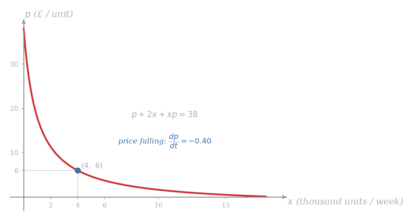
Demand curve p + 2x + xp = 38 plotted as p against x. The curve is steeply decreasing for small x and flattens for large x. The point (4, 6) is marked with reference dotted lines to the axes; an annotation indicates the price is falling at dp/dt = -0.40.

The economic reading of the answer comes from the sign and magnitude. The price drop pulls the market downward along the demand curve from $(4, 6)$ toward larger $x$ . The chain rule converts the price rate, in pounds per week, into a quantity rate, in thousand units per week. Because the demand curve’s slope at $(4, 6)$ is $\dfrac{dp}{dx} = -1{.}6$ (verifiable by implicit differentiation of $(10)$ ), the conversion factor is $\dfrac{dx}{dp} = -1/1{.}6 = -0{.}625$ , giving $\dfrac{dx}{dt} = -0{.}625 \cdot (-0{.}40) = 0{.}25$ , matching the calculation above.

Note (Procedure for related-rates problems)

A related-rates problem typically arrives in plain English with a geometric or economic configuration. Five steps turn it into the algebra of $(11)$ .

Sketch the configuration. Label every quantity that varies; do not label fixed numbers as variables.
Name the variables and pick the independent one. Usually $t$ . Decide which of the named quantities are functions of $t$ and which are constants of the problem.
Find one equation that relates the variables. Geometry, the demand law, the gas law — whatever ties the named quantities together at every instant.
Differentiate the equation with respect to $t$ . Apply the chain rule to every power of a $t$ -dependent variable; apply the product rule to every product of two $t$ -dependent variables.
Substitute the known values and solve for the unknown rate. Substituting before solving is usually faster than solving symbolically and substituting at the end, unless the same problem is asked at multiple instants.

Note (Differentiate before substituting)

The temptation to plug in numbers before differentiating is the single most common error in related-rates problems. Numerical values are true only at one instant; the differentiated equation must describe motion at nearby instants too.

For example, if a circle has radius $r=5$ at one moment, replacing $r$ by $5$ before differentiating would make $r$ look constant and would incorrectly give $\dfrac{dr}{dt}=0$ . Keep the variables as variables, differentiate the relation, and only then substitute the data for the particular instant.

Problem 137

A ladder $5$ meters long leans against a vertical wall. The bottom of the ladder slides away from the wall at a rate of $0{.}3$ meters per second. Let $x$ be the distance from the wall to the foot of the ladder and $y$ the height of the top of the ladder above the ground.

State the equation that relates $x$ and $y$ at every instant. Differentiate it with respect to $t$ and solve symbolically for $\dfrac{dy}{dt}$ in terms of $x$ , $y$ , and $\dfrac{dx}{dt}$ .
Find $\dfrac{dy}{dt}$ at the moment when $x = 3$ meters. Interpret the sign.
Show that, as the foot of the ladder approaches $x = 5$ , the rate $\dfrac{dy}{dt}$ approaches $-\infty$ . Tie this to the geometric statement that the top of the ladder hits the ground at $y = 0$ .

Problem 138

Pollution flows into a circular pond at a steady rate of $0{.}8$ cubic meters per second, spreading uniformly so the surface remains a circle of constant depth $0{.}4$ meters. Let $r$ denote the radius of the spill in meters at time $t$ in seconds.

Express the volume $V$ of polluted water as a function of $r$ alone, using the constant-depth assumption.
Use the chain rule to relate $\dfrac{dV}{dt}$ to $\dfrac{dr}{dt}$ .
Find $\dfrac{dr}{dt}$ at the instant the radius is $5$ meters. Confirm that the rate decreases as $r$ grows, and explain in plain English why the spreading slows even though the inflow is steady.

Problem 139

The price $p$ (in pounds) and weekly sales $x$ (in thousands of units) of a commodity are tied by the demand equation

x^2 + 4 \, x \, p + p^2 = 150.

At a particular moment, $x = 5$ , $p = 5$ , and the manufacturer is raising the price at $\dfrac{dp}{dt} = 0{.}10$ pounds per week.

Differentiate the demand equation with respect to $t$ and solve symbolically for $\dfrac{dx}{dt}$ in terms of $x$ , $p$ , and $\dfrac{dp}{dt}$ .
Compute $\dfrac{dx}{dt}$ at the given instant. State, in plain English, whether sales are rising or falling and by how much.
The total weekly revenue is $R = p \, x$ (in thousand pounds). Use the product rule to compute $\dfrac{dR}{dt}$ at the same instant. Tie the answer to the time-rate machinery from Lesson 4AM.

Problem 140

A spherical balloon is being inflated so that the surface area increases at $\dfrac{dS}{dt} = 12$ square centimeters per second, where $S = 4 \pi r^2$ . The balloon’s volume is $V = \tfrac{4}{3} \pi r^3$ .

Differentiate $S = 4 \pi r^2$ with respect to $t$ and write $\dfrac{dr}{dt}$ in terms of $r$ and $\dfrac{dS}{dt}$ .
Use the chain rule to find $\dfrac{dV}{dt}$ in terms of $r$ and $\dfrac{dS}{dt}$ alone (eliminate $\dfrac{dr}{dt}$ ).
Compute $\dfrac{dV}{dt}$ when $r = 3$ centimeters. Compare with the corresponding calculation in Lesson 4AM’s A balloon inflating example, where the input was $\dfrac{dr}{dt}$ rather than $\dfrac{dS}{dt}$ .

Problem 141

A boat is being pulled toward a dock by a rope passing over a pulley fixed $h = 6$ meters above the water level at the dock. The rope is reeled in at a steady $\dfrac{dL}{dt} = -1$ meter per second, where $L$ is the length of rope from the pulley to the boat (negative because the rope is shortening). Let $x$ be the horizontal distance from the boat to the dock, with $x > 0$ .

Use the right triangle formed by the rope, the pulley height, and the horizontal distance to write the relation $L^{2} = x^{2} + h^{2}$ . Differentiate with respect to $t$ and solve symbolically for $\dfrac{dx}{dt}$ in terms of $x$ , $L$ , and $\dfrac{dL}{dt}$ .
Find $\dfrac{dx}{dt}$ at the moment the boat is $x = 8$ meters from the dock.
Show that $\dfrac{dx}{dt} \to -\infty$ as $x \to 0$ from the positive side. Reconcile this with physical reality: the boat does not actually accelerate to infinite speed at the dock, so where does the model break down?

Why It Works

Implicit differentiation has been used in this lesson without a separate justification, because there isn’t one to give beyond the chain rule of Lesson 4AM. A short derivation makes the reliance explicit.

Proof

Suppose an equation $F(x, y) = 0$ implicitly defines a differentiable function $y = g(x)$ on an interval, in the sense of the Implicit function definition above. Substitute $y = g(x)$ into the equation:

F(x, g(x)) = 0 \quad \text{for every } x \text{ in the interval.}

The left side is a function of $x$ alone, and it is the constant $0$ . Differentiate both sides with respect to $x$ . The right side gives $0$ . The left side, being a composition of $F$ with the pair $(x, g(x))$ , gets differentiated by the chain rule, producing a linear equation in the unknown $g'(x) = \frac{dy}{dx}$ .

Concretely, every term of $F(x, y)$ that contains $y$ alone or in a product with $x$ contributes a $\frac{dy}{dx}$ when differentiated, via the rule $(2)$ applied to powers of $y$ and the product rule applied to $x \cdot y$ products. Every term containing only $x$ contributes nothing involving $\frac{dy}{dx}$ . Collecting and solving for $\frac{dy}{dx}$ — the move named Step 2 through Step 4 of the procedure — completes the calculation.

■

The full statement of the implicit function theorem — which says exactly when an equation $F(x, y) = 0$ defines $y$ as a differentiable function of $x$ near a given solution — is a multivariable result and is left to a later course. For every example in this lesson, the relevant condition holds at every point we sample, and the procedure above produces the slope.

The related-rates version uses the same machinery. If $x = x(t)$ and $y = y(t)$ are differentiable functions of $t$ that satisfy $F(x(t), y(t)) = c$ at every instant, then differentiating both sides with respect to $t$ gives a linear equation in $\dfrac{dx}{dt}$ and $\dfrac{dy}{dt}$ . Each $y$ -power and $x$ -power in $F$ contributes a chain-rule factor; each product $x \, y$ contributes a product-rule pair. If $\dfrac{dx}{dt}$ is nonzero, dividing the related-rates equation by $\dfrac{dx}{dt}$ turns it back into the static slope equation for $\dfrac{dy}{dx}$ . There is no new content, only a different read of the same equation.

Problem 142

A spherical mirror is described by the equation $x^2 + y^2 + z^2 = 25$ in three dimensions. Holding $z = 3$ fixed traces out the latitude curve $x^2 + y^2 = 16$ at that height. Use implicit differentiation on the latitude curve to find $\dfrac{dy}{dx}$ , evaluate it at $(2, 2\sqrt{3})$ , and state the result as a tangent direction in the plane $z = 3$ .

Problem 143

A market’s demand and supply equilibrium for a luxury good is modeled by

p^2 + p q + q^2 = 1200,

where $p$ is the unit price in pounds and $q$ is the quantity sold per week. The curve traces the locus of $(p, q)$ -pairs at which the market clears.

Use implicit differentiation to find $\dfrac{dq}{dp}$ in terms of $p$ and $q$ . (Note the role swap: now $p$ is the independent variable.)
The pair $(p, q) = (20, 20)$ lies on the curve. Compute $\dfrac{dq}{dp}\big|_{(20, 20)}$ and interpret it as a marginal sensitivity in plain English.
State, without further computation, the value of $\dfrac{dp}{dq}$ at the same point, by reciprocity.

Problem 144

For the curve $x^2 - x y + y^2 = 7$ :

Find $\dfrac{dy}{dx}$ by implicit differentiation.
Find the second derivative $\dfrac{d^2 y}{dx^2}$ at the point $(1, 3)$ , by differentiating your answer to part (1) implicitly a second time and substituting both $\dfrac{dy}{dx}\big|_{(1, 3)}$ and the coordinates.
Use the sign of $\dfrac{d^2 y}{dx^2}$ at $(1, 3)$ to say whether the curve is concave up or concave down at that point. Tie the result to the Concavity discussion of Lesson 3AM.