Lesson 4R: Recitation | MA0A: Differentiation

06/03/2026

#Math#Differentiation

Lesson assets

No linked assets.

Lesson 4AM closed with the toolkit table: power, sum, constant multiple, product, quotient, and chain. Any expression assembled from finitely many of those operations is differentiable mechanically. Lesson 4PM removed the last remaining restriction: when the relationship between $x$ and $y$ is given by an equation rather than an explicit formula, the chain rule still produces $\dfrac{dy}{dx}$ as a ratio in $x$ and $y$ , and the same rule converts it into related rates when $t$ is the underlying variable.

Layered Rules in Practice

The hardest part of using the product, quotient, and chain rules together is not the calculus. Every individual derivative is one line. The work is deciding which rule sits on the outside and which sits on the inside.

Example 1 (A three-layer expression)

Differentiate

y = \frac{(2x + 1)^{3}}{\sqrt{x^{2} + 4}}.

The expression is a quotient on the outside, with a power on top and a power-of-a-polynomial on the bottom. Read the architecture before reaching for any rule: outer is quotient, top is a chain $(2x + 1)^{3}$ , bottom is a chain $(x^{2} + 4)^{1/2}$ .

Step 1: derivatives of the two pieces. By the general power rule applied to each composite,

\frac{d}{dx}(2x + 1)^{3} = 3(2x + 1)^{2}(2) = 6(2x + 1)^{2},

\frac{d}{dx}(x^{2} + 4)^{1/2} = \tfrac{1}{2}(x^{2} + 4)^{-1/2}(2x) = \frac{x}{\sqrt{x^{2} + 4}}.

Step 2: assemble with the quotient rule. With $f = (2x + 1)^{3}$ and $g = \sqrt{x^{2} + 4}$ ,

\frac{dy}{dx} = \frac{\sqrt{x^{2} + 4} \cdot 6(2x + 1)^{2} - (2x + 1)^{3} \cdot \dfrac{x}{\sqrt{x^{2} + 4}}}{x^{2} + 4}.

Step 3: clear the inner fraction. Multiply numerator and denominator by $\sqrt{x^{2} + 4}$ :

\frac{dy}{dx} = \frac{6(2x + 1)^{2}(x^{2} + 4) - x(2x + 1)^{3}}{(x^{2} + 4)^{3/2}}.

Step 4: factor. Both terms in the numerator share $(2x + 1)^{2}$ , so

\frac{dy}{dx} = \frac{(2x + 1)^{2}\bigl[6(x^{2} + 4) - x(2x + 1)\bigr]}{(x^{2} + 4)^{3/2}} = \frac{(2x + 1)^{2}(4x^{2} - x + 24)}{(x^{2} + 4)^{3/2}}.

The discriminant of $4x^{2} - x + 24$ is $1 - 384 < 0$ , so the second factor is positive for every real $x$ . Critical numbers come only from $(2x + 1)^{2} = 0$ , giving $x = -\tfrac{1}{2}$ . Since the squared factor is nonnegative on both sides of $-\tfrac{1}{2}$ and the remaining factor is always positive, the slope vanishes there but does not change sign. By the first derivative test, this gives a horizontal tangent but not a relative extremum.

Example 2 (A square-root inside a power)

Differentiate

y = \bigl(\!\sqrt{x^{2} + 1} + 3x\bigr)^{4}.

The outermost rule is the general power rule with $r = 4$ applied to the inner expression $u = \sqrt{x^{2} + 1} + 3x$ :

\frac{dy}{dx} = 4\bigl(\!\sqrt{x^{2} + 1} + 3x\bigr)^{3} \cdot \frac{du}{dx}.

The inner derivative is itself a sum, with the square-root term needing the general power rule a second time:

\frac{du}{dx} = \frac{x}{\sqrt{x^{2} + 1}} + 3 = \frac{x + 3\sqrt{x^{2} + 1}}{\sqrt{x^{2} + 1}}.

Therefore

\frac{dy}{dx} = \frac{4\bigl(\!\sqrt{x^{2} + 1} + 3x\bigr)^{3}\bigl(x + 3\sqrt{x^{2} + 1}\bigr)}{\sqrt{x^{2} + 1}}.

Each new layer of nesting adds one factor: one for the outer power, one for the inner square root. The chain rule applied $n$ times produces $n$ multiplied factors and nothing else.

Problem 1

Differentiate each function. For the first two, simplify until critical numbers are visible without further work.

$y = x\,(x^{2} - 4)^{3}$ .
$y = \!\left(\dfrac{2x - 1}{x^{2} + 1}\right)^{\!4}$ .
$y = \sqrt{\,x + \sqrt{x + \sqrt{x}}\,}\,$ (three-layer chain).

Tangent Lines on Implicit Curves

The static slope formula from Lesson 4PM gives $\dfrac{dy}{dx}$ as a ratio in $x$ and $y$ . When this ratio is finite at the point, it combines with the point-slope form from Lesson 2AM to give the tangent line. In the examples below, a zero denominator with nonzero numerator signals a vertical tangent.

Example 3 (Tangent to a lemniscate)

The curve

(x^{2} + y^{2})^{2} = 8(x^{2} - y^{2}) \tag{1}

is a lemniscate of Bernoulli, the same family as the Lesson 4PM problem (with constants chosen so that the lobes pass through tidy points). A quick check confirms $\bigl(\sqrt{3}, 1\bigr)$ lies on the curve:

(3 + 1)^{2} = 16 = 8(3 - 1).

Find the tangent line there.

Differentiate (1) with respect to $x$ . The left side is a power of a sum; the chain rule gives

2(x^{2} + y^{2})\!\left(2x + 2y\,\frac{dy}{dx}\right) = 16x - 16y\,\frac{dy}{dx}.

Divide both sides by $2$ and expand:

2x(x^{2} + y^{2}) + 2y(x^{2} + y^{2})\frac{dy}{dx} = 8x - 8y\,\frac{dy}{dx}.

Collect $\dfrac{dy}{dx}$ on the left:

\bigl[2y(x^{2} + y^{2}) + 8y\bigr]\frac{dy}{dx} = 8x - 2x(x^{2} + y^{2}),

which factors as

2y\bigl[(x^{2} + y^{2}) + 4\bigr]\frac{dy}{dx} = 2x\bigl[4 - (x^{2} + y^{2})\bigr].

Solve for $\dfrac{dy}{dx}$ :

\frac{dy}{dx} = \frac{x\bigl[4 - (x^{2} + y^{2})\bigr]}{y\bigl[(x^{2} + y^{2}) + 4\bigr]}.

At $\bigl(\sqrt{3}, 1\bigr)$ : $x^{2} + y^{2} = 4$ , so the numerator vanishes and

\left.\frac{dy}{dx}\right|_{(\sqrt{3},\, 1)} = \frac{\sqrt{3}(4 - 4)}{1 \cdot (4 + 4)} = 0.

The tangent at $\bigl(\sqrt{3}, 1\bigr)$ is horizontal, so the line is $y = 1$ . Reading off the slope formula directly: every point on the curve satisfying $x^{2} + y^{2} = 4$ has a horizontal tangent. Geometrically, the lemniscate’s two highest and lowest points sit on the auxiliary circle of radius $2$ .

Remark

The substitution $x^{2} + y^{2} = 4$ collapsed the slope formula to zero in one line. Whenever the curve equation forces a useful value on a sub-expression that appears in $\dfrac{dy}{dx}$ , use it before plugging in numbers.

Higher Derivatives Implicitly

The slope formula from Lesson 4PM is itself an equation in $x$ and $y$ , so a second round of implicit differentiation gives $\dfrac{d^{2}y}{dx^{2}}$ in terms of the same variables.

Example 4 (Second derivative of an ellipse)

For the ellipse $9x^{2} + 4y^{2} = 36$ , find $\dfrac{d^{2}y}{dx^{2}}$ at the point $\bigl(\sqrt{3}, \tfrac{3}{2}\bigr)$ , and use the result to confirm the concavity at that point.

Step 1: first derivative. Differentiate $9x^{2} + 4y^{2} = 36$ implicitly:

18x + 8y\,\frac{dy}{dx} = 0, \qquad \frac{dy}{dx} = -\frac{9x}{4y}. \tag{2}

At $\bigl(\sqrt{3}, \tfrac{3}{2}\bigr)$ : $\dfrac{dy}{dx} = -\dfrac{9\sqrt{3}}{6} = -\dfrac{3\sqrt{3}}{2}$ .

Step 2: second derivative. Differentiate (2) using the quotient rule, treating $\dfrac{dy}{dx}$ as a function of $x$ via $y$ :

\frac{d^{2}y}{dx^{2}} = \frac{d}{dx}\!\left(-\frac{9x}{4y}\right) = -\frac{9}{4} \cdot \frac{y \cdot 1 - x \cdot \dfrac{dy}{dx}}{y^{2}} = -\frac{9}{4} \cdot \frac{y - x\,\dfrac{dy}{dx}}{y^{2}}.

Substitute (2) for $\dfrac{dy}{dx}$ :

\frac{d^{2}y}{dx^{2}} = -\frac{9}{4} \cdot \frac{y - x \cdot \!\left(-\dfrac{9x}{4y}\right)}{y^{2}} = -\frac{9}{4} \cdot \frac{y + \dfrac{9x^{2}}{4y}}{y^{2}} = -\frac{9}{4} \cdot \frac{4y^{2} + 9x^{2}}{4y^{3}}.

The numerator $9x^{2} + 4y^{2}$ equals $36$ on every point of the ellipse, so the second derivative along the curve simplifies to

\frac{d^{2}y}{dx^{2}} = -\frac{9 \cdot 36}{16 y^{3}} = -\frac{81}{4 y^{3}}. \tag{3}

Step 3: evaluate at $\bigl(\sqrt{3}, \tfrac{3}{2}\bigr)$ .

\left.\frac{d^{2}y}{dx^{2}}\right|_{(\sqrt{3},\, 3/2)} = -\frac{81}{4 \cdot (3/2)^{3}} = -\frac{81}{4 \cdot 27/8} = -\frac{81 \cdot 8}{4 \cdot 27} = -6.

Since the second derivative is negative, the upper half of the ellipse is concave down at $\bigl(\sqrt{3}, \tfrac{3}{2}\bigr)$ . This matches the concavity language from Lesson 3AM. Form (3) makes the sign readable: on the upper half ( $y > 0$ ), $\dfrac{d^{2}y}{dx^{2}} < 0$ throughout, so the upper half is concave down everywhere; on the lower half, the sign flips and the curve is concave up.

Problem 2

For the curve $x^{3} + y^{3} = 6xy$ , a scaled folium of Descartes, compute $\dfrac{d^{2}y}{dx^{2}}$ at the point $(3, 3)$ . Explain in one sentence why the answer’s sign matches the geometry of the loop near its top.

Lesson 4PM’s procedure for related rates was: name variables, find one equation tying them together, differentiate with respect to $t$ , then substitute. The next two examples fix the procedure against problems where the equation comes from elementary geometry rather than a model handed across.

Example 5 (A walking pedestrian and a streetlamp)

A streetlamp stands $5$ meters tall. A pedestrian $1{.}8$ meters tall walks away from the foot of the lamp at $\dfrac{dx}{dt} = 1{.}2$ meters per second. How fast is the tip of the pedestrian’s shadow moving along the ground at the moment the pedestrian is $4$ meters from the lamp?

Let $x$ be the pedestrian’s horizontal distance from the lamp post and $s$ the distance from the foot of the lamp to the tip of the shadow. Both $x$ and $s$ are functions of $t$ .

Step 1: write the geometric constraint. The lamp top, the pedestrian’s head, and the tip of the shadow are collinear. The two right triangles they form share the same hypotenuse direction, so by similar triangles,

\frac{s}{5} = \frac{s - x}{1{.}8}.

Cross-multiplying:

1{.}8 s = 5(s - x) = 5s - 5x.

Collecting $s$ ,

3{.}2s = 5x, \qquad s = \frac{5}{3{.}2}\,x = \frac{25}{16}\,x. \tag{4}

The shadow tip is always at a fixed multiple of the pedestrian’s distance, namely $25/16 \approx 1{.}5625$ times.

Step 2: differentiate with respect to $t$ . Equation (4) is linear, so

\frac{ds}{dt} = \frac{25}{16}\,\frac{dx}{dt}.

Step 3: substitute the data. The pedestrian’s distance $x = 4$ never enters because (4) was already simplified to a multiplicative law:

\frac{ds}{dt} = \frac{25}{16}(1{.}2) = 1{.}875 \text{ meters per second.}

The shadow tip moves at 1.875 m/s, faster than the pedestrian.

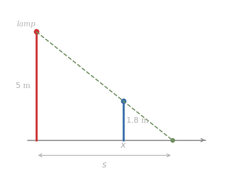
Lamp post of height 5 meters on the left, a pedestrian of height 1.8 meters at horizontal distance x from the lamp, and the tip of the pedestrian's shadow at distance s from the lamp. A dashed light ray runs from the top of the lamp through the top of the pedestrian's head to the ground at the tip of the shadow.

The figure shows why the shadow-tip rate exceeds the pedestrian’s. The light ray to the shadow tip pivots about the lamp top as the pedestrian moves; the pedestrian, whose head sits below that ray, intercepts a shorter arc than the ground does. The ratio $\dfrac{ds/dt}{dx/dt} = \dfrac{5}{5 - 1{.}8} = \dfrac{25}{16}$ depends only on the two heights; the pedestrian’s distance from the lamp drops out.

Remark

The pedestrian’s distance $x = 4$ in this example was a red herring: the constraint (4) is linear in $x$ , so its time derivative carries no instantaneous data. Always carry out Step 2 of the procedure before substituting; if a piece of data turns out to be unnecessary, the structure of the equation will reveal it.

When the geometric constraint is non-linear, the answer depends on the current state of the system in a substantive way.

Example 6 (Water rising in a conical tank)

A water tank has the shape of an inverted right circular cone with height $H = 6$ meters and top radius $R = 3$ meters, so the height is twice the top radius. Water flows in at a steady $\dfrac{dV}{dt} = 0{.}05$ cubic meters per second. How fast is the water level rising at the moment the depth is $h = 2$ meters?

Let $h$ be the depth of water and $r$ the radius of the water surface at depth $h$ . Both vary with time.

Step 1: eliminate $r$ using the tank geometry. The cross-section of the tank is a triangle with $R/H = 3/6 = 1/2$ , so at every depth,

\frac{r}{h} = \frac{1}{2}, \qquad r = \frac{h}{2}.

Step 2: write $V$ as a function of $h$ alone. The volume of water is the volume of a cone of height $h$ and base radius $r = h/2$ :

V = \tfrac{1}{3}\pi r^{2} h = \tfrac{1}{3}\pi\!\left(\frac{h}{2}\right)^{\!2} h = \frac{\pi h^{3}}{12}.

Step 3: differentiate with respect to $t$ . By the chain rule,

\frac{dV}{dt} = \frac{\pi h^{2}}{4}\,\frac{dh}{dt}.

Solve for $\dfrac{dh}{dt}$ :

\frac{dh}{dt} = \frac{4}{\pi h^{2}}\,\frac{dV}{dt}.

Step 4: substitute. At $h = 2$ and $\dfrac{dV}{dt} = 0{.}05$ ,

\frac{dh}{dt} = \frac{4}{4\pi}(0{.}05) = \frac{0{.}05}{\pi} \approx 0{.}0159 \text{ meters per second.}

The water level rises at about 1.59 cm/s when the depth is $2$ meters.

The answer depends on $h$ , and the dependence matters: at depth $h$ , the rate $\dfrac{dh}{dt}$ scales as $1/h^{2}$ , so the level rises four times faster at depth $1$ than at depth $2$ , and nine times faster at depth $1$ than at depth $3$ . The shallow water has a small surface, so a fixed inflow stretches further upward; deep water has a wide surface, so the same inflow spreads sideways before it can lift the level. Substituting before differentiating, contrary to Lesson 4PM’s Differentiate before substituting note, would remove this $h$ -dependence and give the wrong rate.

Problem 3

A second tank has the shape of an inverted cone with height $H = 4$ meters and top radius $R = 2$ meters. Water flows out of a small hole at the bottom at a rate proportional to the depth: $\dfrac{dV}{dt} = -k h$ for some constant $k > 0$ , where $h$ is the current water depth.

Express $V$ in terms of $h$ alone using the similar-triangle ratio between the water surface radius and the depth, as in the Water rising in a conical tank example.
Use the chain rule to find $\dfrac{dh}{dt}$ in terms of $h$ , $k$ , and the geometric constants. Simplify to a single expression with no $V$ or $r$ remaining.
Describe what happens to the formula as $h$ approaches $0$ from above, and explain why this proportional-outflow model stops being physically reliable near an empty tank.

The examples above track rates after the formula is already known. The next question is different: which functions have a rate of change proportional to their current value?

Preview for Lesson 5: Exponential Functions

Three basic models motivate the next function family. The full derivative rules for exponential functions are developed in Lesson 5; here the goal is only to identify the kind of model that needs them.

When an investment grows by a fixed percentage each year, the yearly increase is proportional to the current balance: the larger the balance, the larger the next increase in pounds. When a bacteria culture grows in a nutrient-rich Petri dish, the rate of growth at any moment is proportional to the number of bacteria currently present. A pile of radioactive uranium $^{235}\mathrm{U}$ decays at a rate that, at every moment, is proportional to the amount of $^{235}\mathrm{U}$ still present. The first two are instances of exponential growth; the third, of exponential decay.

What ties them together is a structural condition the toolkit rules cannot meet. A nonconstant function $f(t)$ whose rate of change satisfies $f'(t) = k \, f(t)$ with nonzero constant $k$ cannot be a polynomial: every nonconstant polynomial’s derivative is one degree lower than itself, so $f'$ is not a nonzero constant multiple of $f$ . Nor can it be a rational function for the simple examples we want here. A new family of functions is required.

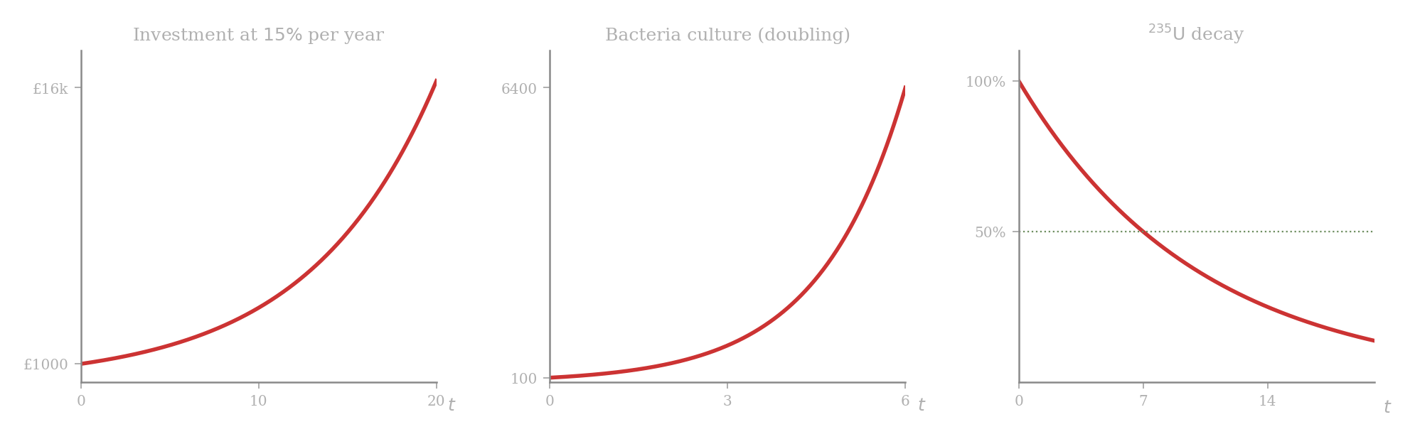
Three small panels side by side. Left: a 15% per year investment, with the balance rising along a curve whose slope grows with the balance. Center: a bacteria population doubling at a steady rate, plotted on a vertical axis. Right: a pile of radioactive uranium-235 decaying, with the mass falling along a curve whose magnitude of slope shrinks as the mass shrinks. All three panels share the same time axis.

The three panels share a single shape: a curve whose vertical rate at every point is proportional to its current height, rising in the first two cases and falling in the third. The function family that produces this shape is the family of exponential functions.

Definition

Throughout this section, $b$ denotes a positive number with $b \neq 1$ .

Definition 1 (Exponential Function)

The exponential function with base $b$ is

f(x) = b^{x},

defined for every real number $x$ . The number $b > 0$ , $b \neq 1$ is the base.

The variable sits in the exponent. That placement is what distinguishes exponential functions from the power functions $x^{r}$ whose derivatives were studied in Lesson 2PM, where the variable was the base and the exponent was a fixed constant. Swapping the two roles changes nearly everything: the toolkit rule for $x^{r}$ does not apply to $b^{x}$ , the shape of the graph is qualitatively different, and the rate of change is proportional to the function itself.

For integer and rational exponents, we use the usual meanings:

b^{0} = 1, \qquad b^{n} = \underbrace{b \cdot b \cdots b}_{n \text{ factors}}, \qquad b^{-n} = \frac{1}{b^{n}}, \qquad b^{1/n} = \sqrt[n]{b}, \qquad b^{p/q} = (\sqrt[q]{b})^{p}.

For irrational exponents such as $x = \sqrt{3}$ or $x = \pi$ , one defines $b^{x}$ by approximating $x$ with rational numbers and taking a limit; the details are omitted here, and we assume that $b^{x}$ is defined for every real $x$ in such a way that the laws of exponents below hold without exception.

Laws of Exponents

The six laws of exponents transfer unchanged from rational exponents to real exponents.

Theorem 1 (Laws of Exponents)

For positive numbers $a, b$ and real numbers $x, y$ :

(i) $b^{x} \cdot b^{y} = b^{x + y}$

(ii) $b^{-x} = \dfrac{1}{b^{x}}$

(iii) $\dfrac{b^{x}}{b^{y}} = b^{x - y}$

(iv) $(b^{y})^{x} = b^{xy}$

(v) $a^{x} \cdot b^{x} = (ab)^{x}$

(vi) $\dfrac{a^{x}}{b^{x}} = \!\left(\dfrac{a}{b}\right)^{\!x}$

Three of these laws, (i), (ii), and (iv), do much of the work. Law (iii) is law (i) combined with law (ii), while laws (v) and (vi) record how a common exponent distributes across multiplication and division of positive bases. Memorizing the six is faster than re-deriving each, but knowing which law is being used keeps the algebra honest.

Property (iv) is the one that earns its keep most often: it converts powers of one base into powers of another, provided the bases share a common smaller base. For example,

8^{x} = (2^{3})^{x} = 2^{3x}, \qquad \!\left(\tfrac{1}{9}\right)^{\!x} = (3^{-2})^{x} = 3^{-2x}, \qquad 27^{x/3} = (3^{3})^{x/3} = 3^{x}.

This is the conversion that makes a comparison of two seemingly different exponentials possible at all.

Example 7 (Rewriting in a common base)

Use the laws of exponents to write each expression in the form $2^{kx}$ for a suitable constant $k$ .

$4^{5x/2}$
$\bigl(2^{4x} \cdot 2^{-x}\bigr)^{1/2}$
$8^{x/3} \cdot 16^{3x/4}$
$\dfrac{10^{x}}{5^{x}}$

Solution. Each part picks out one or two of the six laws.

Replace the base $4 = 2^{2}$ and apply law (iv):

4^{5x/2} = (2^{2})^{5x/2} = 2^{2 \cdot (5x/2)} = 2^{5x}.

Combine the two factors inside the parentheses using law (i), then law (iv):

(2^{4x} \cdot 2^{-x})^{1/2} = (2^{4x - x})^{1/2} = (2^{3x})^{1/2} = 2^{(3/2) x}.

Replace $8 = 2^{3}$ and $16 = 2^{4}$ , apply law (iv) to each factor, and finish with law (i):

8^{x/3} \cdot 16^{3x/4} = (2^{3})^{x/3} \cdot (2^{4})^{3x/4} = 2^{x} \cdot 2^{3x} = 2^{4x}.

Two routes. First, apply law (v) to $10^{x} = (2 \cdot 5)^{x} = 2^{x} \cdot 5^{x}$ , then cancel:

\frac{10^{x}}{5^{x}} = \frac{2^{x} \cdot 5^{x}}{5^{x}} = 2^{x}.

Alternatively, apply law (vi) directly:

\frac{10^{x}}{5^{x}} = \!\left(\frac{10}{5}\right)^{\!x} = 2^{x}.

Both routes land on $2^{x} = 2^{1 \cdot x}$ , so $k = 1$ . The two-route check is structural rather than numerical: if the two laws (v) and (vi) ever produced different answers, one of them would be wrong.

Problem 4

Write each expression in the form $3^{kx + c}$ for suitable constants $k$ and $c$ .

$9^{x + 1}$ .
$\!\left(\tfrac{1}{27}\right)^{\!2x}$ .
$\dfrac{81^{x/2}}{3^{x}}$ .
$\!\left(9^{x} \cdot 27^{x/3}\right)^{2}$ .

Problem 5

Rewrite each expression as a single exponential $b^{x}$ for the smallest possible integer base $b > 1$ .

$4^{x} \cdot 8^{x}$ .
$\dfrac{6^{x}}{3^{x}}$ .
$\dfrac{2^{2x} \cdot 9^{x}}{6^{x}}$ .

Example 8 (A compound interest balance)

A British investor places £1000 into an account paying $15\%$ annual interest, compounded once per year. After $t$ years, the balance is

B(t) = 1000 \cdot (1{.}15)^{t}.

Without the laws of exponents, the question “what is the balance after $20$ years?” is answered only by computing $1000 \cdot (1{.}15)^{20}$ directly. With them, one can also write the same balance using a different base. Using law (iv) with $1{.}15 = (1{.}15^{1/4})^{4}$ , the balance can be rewritten in quarterly steps:

B(t) = 1000 \cdot \bigl((1{.}15)^{1/4}\bigr)^{4t} \approx 1000 \cdot (1{.}03556)^{4t}.

The exact equivalent quarterly growth factor is $(1{.}15)^{1/4}$ , whose decimal approximation is $1{.}03556$ . An account multiplying by this exact factor each quarter compounds to the same yearly $15\%$ . The two formulas describe the same balance at every $t$ , but expose different operational pieces, yearly versus quarterly, by a single application of law (iv). The yearly increase is still $15\%$ of the current balance at each annual compounding step; the base only changes how the same multiplication is recorded.

Problem 6

A radioactive sample’s mass after $t$ years is modeled by

M(t) = M_{0} \cdot (0{.}5)^{t / T},

where $T > 0$ is the half-life in years and $M_{0}$ is the initial mass. Verify two structural properties from the laws of exponents alone, without doing any numerical calculation:

$M(0) = M_{0}$ and $M(T) = M_{0}/2$ .
The mass at time $t + T$ is exactly half the mass at time $t$ , for every $t$ .

State, in plain English, what property (2) says about the model.

Graphs

The qualitative shape of $y = b^{x}$ is fixed by the value of $b$ relative to $1$ .

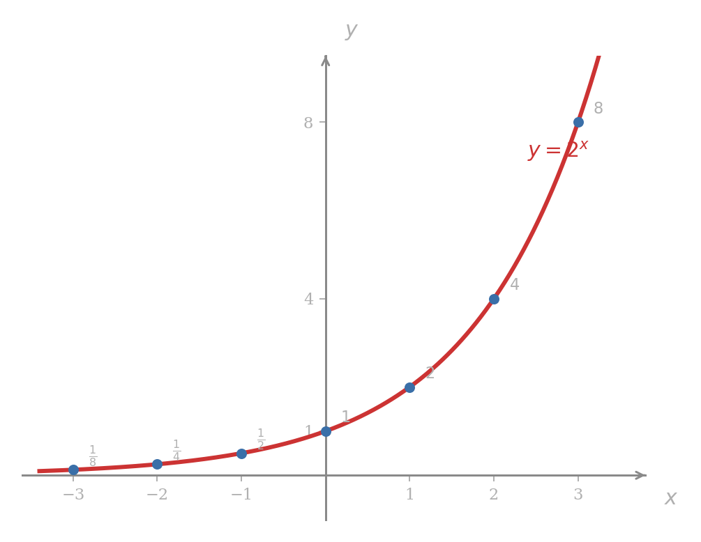
The case $b = 2$ tabulates cleanly. Sample values:

2^{-3} = \tfrac{1}{8}, \qquad 2^{-2} = \tfrac{1}{4}, \qquad 2^{-1} = \tfrac{1}{2}, \qquad 2^{0} = 1, \qquad 2^{1} = 2, \qquad 2^{2} = 4, \qquad 2^{3} = 8.

Plotting the seven points and joining them by a smooth curve produces the now-standard exponential shape: increasing, passing through $(0, 1)$ , approaching the $x$ -axis on the left as $x \to -\infty$ , and growing without bound on the right as $x \to \infty$ .

Graph of y equals 2 to the x. Seven sample points are marked at x equals minus three through positive three with their y-values. The curve passes smoothly through them, crossing the y-axis at one, approaching the x-axis as a horizontal asymptote on the left, and rising steeply on the right.

Two features of the graph carry over to every base $b > 1$ .

The graph passes through $(0, 1)$ , since $b^{0} = 1$ for every positive $b$ .
The graph never touches the $x$ -axis: $b^{x} > 0$ for every real $x$ , so the line $y = 0$ is a horizontal asymptote on the left (in the sense of Lesson 3AM’s Intercepts, Undefined Points, and Asymptotes discussion) but is never reached.

The third feature, that the graph is everywhere increasing, also carries over for $b > 1$ , but the speed of the increase is base-dependent.

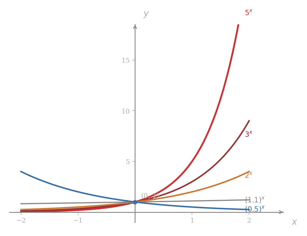
Five exponential curves drawn on the same axes for x between minus two and two. The increasing curves y equals 5 to the x, y equals 3 to the x, y equals 2 to the x, and y equals 1.1 to the x become steeper as the base grows. The curve y equals 0.5 to the x is decreasing and reflects y equals 2 to the x across the y-axis. All five pass through the point (0, 1).

The figure compares five curves at once. Among the increasing curves, reading from steepest to flattest at $x = 0$ gives

y = 5^{x}, \qquad y = 3^{x}, \qquad y = 2^{x}, \qquad y = (1{.}1)^{x}.

These four are increasing because their bases satisfy $b > 1$ . The curve $y = (0{.}5)^{x}$ is decreasing because its base satisfies $0 < b < 1$ . Among the increasing curves, the steepness at $x = 0$ grows with the base: a small change in $x$ near zero produces a much larger change in $5^{x}$ than in $(1{.}1)^{x}$ , because larger bases multiply by more for each unit gained.

The case $0 < b < 1$ produces decreasing curves rather than increasing ones, but is structurally not new: by law (ii),

\!\left(\tfrac{1}{b}\right)^{\!x} = b^{-x},

so the graph of $y = (0{.}5)^{x}$ is the reflection of $y = 2^{x}$ across the $y$ -axis. Studying $b > 1$ alone covers $0 < b < 1$ by reflection.

The Injectivity Property

Every exponential graph in the previous figure has the same structural feature: it is strictly monotonic. For $b > 1$ it is strictly increasing; for $0 < b < 1$ it is strictly decreasing. In either case, no horizontal line crosses the graph twice. Equivalently, an exponential function is one-to-one: distinct inputs produce distinct outputs.

Theorem 2 (Injectivity of

b^{x}

)

For any positive number $b$ with $b \neq 1$ , the equation

b^{r} = b^{s}

implies $r = s$ .

The result is the algebraic shadow of the geometric monotonicity. If $b > 1$ and $r < s$ , then $b^{s} = b^{r} \cdot b^{s-r}$ with $b^{s-r} > 1$ , since the exponent $s - r$ is positive. Thus $b^{s} > b^{r}$ , and the two values cannot coincide. The case $0 < b < 1$ runs the same argument with the inequality flipped. The base $b = 1$ is excluded precisely because $1^{r} = 1^{s} = 1$ for every $r$ and $s$ ; the only base that fails injectivity is the one we ruled out from the start.

Example 9 (Solving an exponential equation)

Find every $x$ for which $3^{5x} = 27$ .

The right-hand side is a power of the same base: $27 = 3^{3}$ . The equation becomes

3^{5x} = 3^{3}.

By injectivity, the exponents must be equal:

5x = 3, \qquad x = \tfrac{3}{5}.

The single root is forced. The structure of exponential functions reduces an equation in the exponent to a linear equation in $x$ .

Example 10 (When the bases differ on first inspection)

Find every $x$ for which $4^{x + 1} = \!\left(\tfrac{1}{8}\right)^{\!x - 2}$ .

Neither side is in a common base immediately, but both $4$ and $\tfrac{1}{8}$ are powers of $2$ :

4 = 2^{2}, \qquad \tfrac{1}{8} = 2^{-3}.

Apply law (iv) to each side:

(2^{2})^{x + 1} = (2^{-3})^{x - 2}, \qquad 2^{2(x+1)} = 2^{-3(x-2)}.

By injectivity,

2(x + 1) = -3(x - 2),

2x + 2 = -3x + 6,

5x = 4, \qquad x = \tfrac{4}{5}.

The conversion to a common base via law (iv) is the only non-trivial content; injectivity then leaves a linear equation.

Example 11 (A quadratic equation in disguise)

Find every $x$ for which $9^{x} - 4 \cdot 3^{x} + 3 = 0$ .

The expression is a polynomial in $3^{x}$ , not in $x$ itself: by law (iv), $9^{x} = (3^{2})^{x} = (3^{x})^{2}$ . Set $u = 3^{x}$ . The equation becomes

u^{2} - 4 u + 3 = 0.

Factor: $(u - 1)(u - 3) = 0$ , so $u = 1$ or $u = 3$ . Translate each back through $u = 3^{x}$ :

$3^{x} = 1 = 3^{0}$ , so $x = 0$ by injectivity.
$3^{x} = 3 = 3^{1}$ , so $x = 1$ by injectivity.

Both roots check in the original equation: $9^{0} - 4 \cdot 3^{0} + 3 = 1 - 4 + 3 = 0$ , and $9^{1} - 4 \cdot 3^{1} + 3 = 9 - 12 + 3 = 0$ .

The substitution $u = 3^{x}$ is the useful move. Whenever an equation contains $9^{x}$ , $3^{x}$ , and constants, one substitution turns it into a polynomial equation in $u$ . Any root of that polynomial that lies in $u > 0$ corresponds, by injectivity, to a single $x$ .

Remark

The substitution $u = 3^{x}$ in the example above is admissible only because $3^{x} > 0$ for every real $x$ . Roots of the polynomial in $u$ that fall in $u \leq 0$ correspond to no real $x$ . If the polynomial above had been $u^{2} + 4u + 3 = (u + 1)(u + 3)$ , both roots $u = -1$ and $u = -3$ would have been spurious, and the original exponential equation would have no real solution. Always check the sign of every polynomial root before translating back.

Problem 7

Solve each equation for $x$ , using the injectivity property and the laws of exponents as needed.

$5^{x + 2} = 125$ .
$2^{3x - 1} = 16^{x}$ .
$9^{x} = 27^{x - 2}$ .
$\!\left(\tfrac{1}{4}\right)^{\!x} = 8^{x + 5}$ .

Problem 8

Solve each quadratic-in-disguise equation by an appropriate substitution. Discard any root of the substituted equation that does not correspond to a real $x$ .

$4^{x} - 5 \cdot 2^{x} + 4 = 0$ .
$25^{x} - 6 \cdot 5^{x} + 5 = 0$ .
$9^{x} + 3^{x + 1} = 4$ . (Hint: the term $3^{x + 1} = 3 \cdot 3^{x}$ .)

Problem 9

A British investor’s account balance is $B(t) = 1000 \cdot (1{.}15)^{t}$ pounds after $t$ years. Suppose a quarterly growth factor is chosen to be exactly $(1{.}15)^{1/4}$ . After how many years does the balance reach

1000 \cdot (1{.}15)^{10} \cdot \bigl((1{.}15)^{1/4}\bigr)^{8}

pounds? Use the laws of exponents to convert the right-hand side into the form $1000 \cdot (1{.}15)^{T}$ and solve for $T$ by injectivity.

Reading the Slope

A single qualitative observation about the graphs of $b^{x}$ ties the algebra above back to the proportionality $f' = k\,f$ that opened this half of the recitation.

For every $b > 1$ , the graph of $y = b^{x}$ is concave up everywhere. Reading from left to right, the slope is small and positive on the far left, becomes moderate near $x = 0$ , and grows on the far right. Lesson 5 will make the following preview precise: the slope at $x = -1$ is $1/b$ times the slope at $x = 0$ , the slope at $x = 1$ is $b$ times the slope at $x = 0$ , and so on. The slope at every $x$ is a constant multiple of the slope at $0$ , with the constant equal to $b^{x}$ itself.

The proportionality $f' = k \, f$ is the formula this preview is pointing toward. The constant $k$ is whatever the slope of $b^{x}$ happens to be at $x = 0$ , and Lesson 5 turns that observation into a derivative formula.

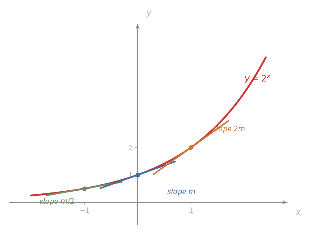
Three tangent lines drawn on the graph of y equals 2 to the x at x equals minus one, x equals zero, and x equals one. The middle tangent is labelled with slope m, while the other two are labelled with the Lesson 5 preview pattern m over 2 and 2m.

Three tangent lines, drawn at $x = -1$ , $x = 0$ , and $x = 1$ on the graph of $y = 2^{x}$ , have slopes

\frac{m}{2}, \qquad m, \qquad 2 m,

where $m$ is the slope at $x = 0$ . The middle slope is the lone unknown. Once it is named, every other slope is read off as $m \cdot 2^{x}$ in the Lesson 5 formula.

Exercises

Exercise 1

Differentiate $y = (x^{2} + 1)^{4}(2x - 3)^{5}$ using the product rule and the general power rule. Factor the answer over the integers. Identify every $x$ for which $y' = 0$ .

Exercise 2

For the curve $x^{2} - 3xy + y^{2} = 11$ :

Use implicit differentiation to find $\dfrac{dy}{dx}$ as a function of $x$ and $y$ .
Show that the point $(2, -1)$ lies on the curve, and compute the tangent slope there.
Find the equation of the tangent line at $(2, -1)$ in the form $y = mx + b$ .

Exercise 3

Differentiate

f(x) = \sqrt{\frac{x^{2} + 1}{x^{2} - 1}}

on the domain $|x| > 1$ by writing $f$ as a power and combining the general power rule with the quotient rule. Express the answer with no negative exponents and identify any $x$ at which $f'(x) = 0$ .

Exercise 4

A spherical balloon’s radius is increasing at $\dfrac{dr}{dt} = 0{.}3$ centimeters per second. Air is being pumped in at a rate $\dfrac{dV}{dt}$ that is not constant; it increases as the balloon grows. Find $\dfrac{dV}{dt}$ at the moment $r = 5$ cm. Then explain why a constant rate of radial growth requires a non-constant rate of volume supply, citing the chain rule.

Exercise 5

A 13-foot ladder leans against a vertical wall. The bottom slips away from the wall at $0{.}5$ feet per second.

Find the rate at which the top of the ladder is sliding down the wall when the bottom is $5$ feet from the wall.
The area of the triangle enclosed by the ladder, the wall, and the ground is $A = \tfrac{1}{2}xy$ . Find $\dfrac{dA}{dt}$ at the same instant.
At what value of $x$ is the area $A$ momentarily constant, meaning $\dfrac{dA}{dt} = 0$ ? Interpret in plain English.

Exercise 6

For the demand curve $p^{2} + 2pq + 2q^{2} = 250$ , where $p$ is unit price (pounds) and $q$ is quantity sold (thousand units per week):

Use implicit differentiation to find $\dfrac{dq}{dp}$ in terms of $p$ and $q$ .
The point $(p, q) = (10, 5)$ lies on the curve. Compute $\dfrac{dq}{dp}$ there and state, in plain English, what the answer says about price sensitivity.
The total weekly revenue is $R = pq$ . Use the product rule on $R(t) = p(t) q(t)$ to find $\dfrac{dR}{dt}$ at the instant $(p, q) = (10, 5)$ and $\dfrac{dp}{dt} = 0{.}2$ pounds per week.

Exercise 7

Show that for any differentiable curve $F(x, y) = 0$ implicitly defining $y$ as a function of $x$ near a point $(a, b)$ with $\dfrac{dy}{dx}\big|_{(a, b)} = m$ , the normal line at $(a, b)$ , meaning the line through $(a, b)$ perpendicular to the tangent, has equation

y - b = -\frac{1}{m}(x - a)

when $m \neq 0$ , and $x = a$ when $m = 0$ . Apply this to the circle $x^{2} + y^{2} = 25$ at the point $(3, 4)$ to find both the tangent line and the normal line, and verify that the normal line passes through the origin.

Exercise 8

Write each expression as a single exponential of the form $2^{kx + c}$ or $3^{kx + c}$ for suitable constants $k$ and $c$ .

$4^{x + 1} \cdot 8^{x - 2}$ .
$\dfrac{27^{x}}{9^{x - 1}}$ .
$\!\left(2^{x} \cdot 4^{x + 1}\right)^{1/2}$ .

Exercise 9

Solve each exponential equation for $x$ . State whether each step uses a law of exponents (and which one) or the injectivity property.

$2^{x^{2}} = 16^{x}$ .
$3^{x + 1} + 3^{x} = 36$ .
$5^{2x} - 26 \cdot 5^{x} + 25 = 0$ .

Exercise 10

A pile of $^{14}\mathrm{C}$ has half-life $T = 5730$ years. The mass remaining after $t$ years is $M(t) = M_{0} \cdot (0{.}5)^{t / T}$ .

Use the laws of exponents to show that $M(t + T) = \tfrac{1}{2} M(t)$ for every $t$ .
Express $M(t)$ in the form $M_{0} \cdot 2^{-t/T}$ using law (ii).
Find the value of $t$ at which exactly $\tfrac{1}{8}$ of the original mass remains, by setting up an equation in the form $2^{-t/T} = 2^{-k}$ and applying injectivity.

Exercise 11

The graph of $y = b^{x}$ passes through $(0, 1)$ for every admissible $b$ . Determine the unique base $b > 0$ for which the graph also passes through $(2, 9)$ . Then use that $b$ to compute the value of the function at $x = 1/2$ and at $x = -3$ .

Exercise 12

Show, using the laws of exponents alone, that for every positive $b$ with $b \neq 1$ and every real $x$ ,

b^{x} \cdot b^{-x} = 1.

Conclude that $b^{x}$ and $b^{-x}$ are reciprocals. Use this to prove that the graph of $y = b^{x}$ never crosses the $x$ -axis, without appealing to the definition of $b^{x}$ for irrational $x$ .

Lesson assets

Implicit Differentiation, Related Rates, and Exponential Functions

Layered Rules in Practice

Tangent Lines on Implicit Curves

Higher Derivatives Implicitly

Related Rates I: Geometry of a Shadow

Related Rates II: A Conical Tank

Preview for Lesson 5: Exponential Functions

Definition

Laws of Exponents

Graphs

The Injectivity Property

Reading the Slope

Exercises