02/03/2026

#Math#Differentiation

Video

Lesson assets

video link

CS50P Lecture 0: Functions, Variables

exercise

Exercise 4 PDF

Differentiation Techniques: Product, Quotient, and chain rules

The differentiation rules from Lesson 2PM and Recitation 2 — power, sum, constant multiple, general power — handle every polynomial we wrote down in Lesson 3. They run out the moment two functions are multiplied together, divided by one another, or composed in a way not already covered by the general power rule. Three expressions flag the gap:

F(x) = (x^2 - 1)^4 (x^2 + 1)^5, \qquad G(x) = \frac{x^3}{(x^2 + 1)^4}, \qquad H(x) = \sqrt{4 x^2 + 1}.

The first is a product, the second a ratio, the third a composition. Brute expansion of $F$ has many terms, and the answer we want, $F'$ , factors back into a clean form anyway. Re-writing $G$ as $x^3 (x^2 + 1)^{-4}$ turns the ratio into a product but does not remove the need for a product rule. The expression $H$ can be handled by the general power rule because the outside function is a half-power; the full chain rule explains why that same outside-inside pattern works beyond powers.

This lesson develops three rules in turn: the product rule for expressions like $F$ , the quotient rule for expressions like $G$ , and the chain rule for expressions like $H$ . The chain rule turns out to be the umbrella under which the general power rule and the quotient-rule proof both sit; once it is in hand, every expression built from finitely many sums, differences, products, quotients, and compositions of differentiable elementary pieces is itself differentiable.

When the Naive Guess Fails

The sum rule stated that the derivative of a sum is the sum of the derivatives. A natural reflex is to try the same for products: guess that $\frac{d}{dx}[f(x) g(x)] = f'(x) g'(x)$ . A single counterexample buries the guess.

Take $f(x) = x^2$ and $g(x) = x^3$ . Their product is $x^5$ , and the power rule gives

\frac{d}{dx}(x^5) = 5 x^4.

The naive guess gives $f'(x) g'(x) = (2 x)(3 x^2) = 6 x^3$ . Not even the same degree. Whatever the correct rule is, it must mix $f$ , $g$ , $f'$ , and $g'$ in a more substantial way.

The rectangle picture below explains why. If $f(x)$ and $g(x)$ are the side lengths of a rectangle, then the product $f(x) g(x)$ is its area. Increase $x$ slightly, so that $f$ grows by $\Delta f$ and $g$ grows by $\Delta g$ . The new area decomposes into four rectangles: the original $fg$ , a thin top strip of area $f \, \Delta g$ , a thin right strip of area $g \, \Delta f$ , and a tiny corner of area $\Delta f \, \Delta g$ .

Rectangle of sides f(x) and g(x) enlarged by Δf horizontally and Δg vertically. The change in area decomposes into a top strip f·Δg, a right strip g·Δf, and a small corner Δf·Δg.

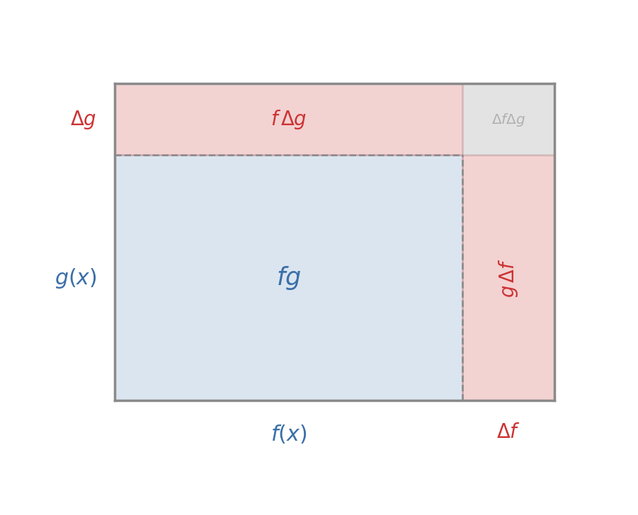
The change in area is $f \, \Delta g + g \, \Delta f + \Delta f \, \Delta g$ . Dividing by the change in input $h$ and letting $h \to 0$ , the corner term carries an extra factor of $h$ and vanishes, leaving exactly $f \, g' + g \, f'$ . The naive guess corresponds to the corner alone, which is precisely the term that drops out.

The Product Rule

Theorem 13 (Product Rule)

If $f$ and $g$ are differentiable at $x$ , then so is the product $fg$ , and

\frac{d}{dx}\bigl[f(x) \, g(x)\bigr] = f(x) \, g'(x) + g(x) \, f'(x).

In words: the derivative of a product is the first function times the derivative of the second, plus the second function times the derivative of the first.

Proof

Let $P(x) = f(x) \, g(x)$ . By the limit definition of the derivative,

P'(x) = \lim_{h \to 0} \frac{f(x+h) \, g(x+h) - f(x) \, g(x)}{h}.

Add and subtract $f(x+h) \, g(x)$ in the numerator:

\begin{aligned} P'(x) &= \lim_{h \to 0} \frac{f(x+h)\,g(x+h) - f(x+h)\,g(x) + f(x+h)\,g(x) - f(x)\,g(x)}{h}\\ &= \lim_{h \to 0} \left[ f(x+h) \cdot \frac{g(x+h) - g(x)}{h} + g(x) \cdot \frac{f(x+h) - f(x)}{h} \right]. \end{aligned}

The two difference quotients tend to $g'(x)$ and $f'(x)$ . Because $f$ is differentiable at $x$ , it is continuous there (Lesson 2PM), so $\lim_{h \to 0} f(x+h) = f(x)$ . Splitting the limit of the sum into a sum of limits and the limit of the product into a product of limits (both moves justified because every individual limit exists),

P'(x) = f(x) \, g'(x) + g(x) \, f'(x).

■

The trick of adding and subtracting $f(x+h) \, g(x)$ is what isolates the two strips in the rectangle picture. Without that intermediate step, $f$ and $g$ change together inside a single difference quotient, and the rules from Lesson 2 do not separate them.

Example 102 (Verifying the product rule)

For $f(x) = x^2$ and $g(x) = x^3$ , the product rule should reproduce $\frac{d}{dx}(x^5) = 5 x^4$ . Compute

\begin{aligned} \frac{d}{dx}(x^2 \cdot x^3) &= x^2 \cdot \frac{d}{dx}(x^3) + x^3 \cdot \frac{d}{dx}(x^2)\\ &= x^2 (3 x^2) + x^3 (2 x)\\ &= 3 x^4 + 2 x^4 = 5 x^4. \checkmark \end{aligned}

The rule recovers the answer the power rule already supplied. The genuine work begins where the power rule alone cannot reach.

Example 103 (A polynomial product, kept factored)

Differentiate $y = (2 x^3 - 5 x)(3 x + 1)$ .

Set $f(x) = 2 x^3 - 5 x$ and $g(x) = 3 x + 1$ . Then $f'(x) = 6 x^2 - 5$ and $g'(x) = 3$ , so

\begin{aligned} \frac{dy}{dx} &= (2 x^3 - 5 x)(3) + (3 x + 1)(6 x^2 - 5)\\ &= 6 x^3 - 15 x + 18 x^3 - 15 x + 6 x^2 - 5\\ &= 24 x^3 + 6 x^2 - 30 x - 5. \end{aligned}

Multiplying out the original product first and then differentiating term by term gives the same answer. The product rule simply skips the algebra.

Remark

The product rule is symmetric: $f \, g' + g \, f' = g \, f' + f \, g'$ . Some texts state it the other way round. Pick one ordering and keep it: the first function times the derivative of the second, plus the second function times the derivative of the first. Mixing orderings inside one calculation is where signs get lost.

Problem 102

Differentiate $y = (4 x^3 + x)(7 - x^2)$ using the product rule. Leave the answer in the unsimplified form first, then expand and collect like terms. Verify by multiplying the two factors out before differentiating.

Problem 103

A rectangular sheet of metal expands under heat. After $t$ seconds, its length is $L(t) = 12 + 0{.}03 \, t$ centimeters and its width is $W(t) = 8 + 0{.}02 \, t$ centimeters. The area is $A(t) = L(t) \, W(t)$ .

Without expanding, write $A'(t)$ using the product rule.
Compute $A'(0)$ . Which side contributes more to the initial rate of growth, length or width? Tie the answer to the rectangle picture in When the Naive Guess Fails.

Recovering the General Power Rule

Apply the product rule to a function multiplied by itself.

Example 104 (A function squared)

Apply the product rule to $y = g(x) \cdot g(x)$ :

\frac{d}{dx}\bigl[g(x) \cdot g(x)\bigr] = g(x) \cdot g'(x) + g(x) \cdot g'(x) = 2 \, g(x) \, g'(x).

The general power rule, applied to the same expression $[g(x)]^2$ , gives $2 \, g(x) \, g'(x)$ . The two rules agree.

For positive integer powers, the general power rule agrees with what the product rule would give if we applied it repeatedly to $g \cdot g \cdot \cdots \cdot g$ . Recitation 2 stated the general power rule more broadly, including fractional and negative rational powers, so the product rule does not replace it. The point is narrower but useful: when a product contains powers of differentiable expressions, the two rules are designed to fit together.

Combining the Product Rule with the General Power Rule

The product rule rarely arrives alone. Most product expressions involve composite pieces, and the general power rule supplies $f'$ and $g'$ for those pieces.

Example 105 (Differentiate and simplify)

Find $\dfrac{dy}{dx}$ where $y = (x^2 - 1)^4 (x^2 + 1)^5$ .

Set $f(x) = (x^2 - 1)^4$ and $g(x) = (x^2 + 1)^5$ . Apply the general power rule to each:

f'(x) = 4 (x^2 - 1)^3 (2 x), \qquad g'(x) = 5 (x^2 + 1)^4 (2 x).

By the product rule,

\frac{dy}{dx} = (x^2 - 1)^4 \cdot 5 (x^2 + 1)^4 (2 x) + (x^2 + 1)^5 \cdot 4 (x^2 - 1)^3 (2 x). \tag{1}

Equation $(1)$ is sufficient if the goal is a numerical value at a single point — substituting $x = 2$ is straightforward. The work begins when the goal is to find where the derivative vanishes, because $(1)$ as written is a sum of two products, not one expression set equal to zero.

Both terms share $2 x$ , a power of $(x^2 - 1)$ , and a power of $(x^2 + 1)$ . The largest factor common to both is $2 x (x^2 - 1)^3 (x^2 + 1)^4$ . Pulling it out,

\frac{dy}{dx} = 2 x (x^2 - 1)^3 (x^2 + 1)^4 \bigl[5 (x^2 - 1) + 4 (x^2 + 1)\bigr].

The bracketed factor simplifies: $5 x^2 - 5 + 4 x^2 + 4 = 9 x^2 - 1$ . Hence

\frac{dy}{dx} = 2 x (x^2 - 1)^3 (x^2 + 1)^4 (9 x^2 - 1). \tag{2}

Form $(2)$ exposes every critical number at a glance: $\frac{dy}{dx} = 0$ when $x = 0$ , $x = \pm 1$ , or $9 x^2 = 1$ (giving $x = \pm 1/3$ ). The same information was buried inside $(1)$ but not visible.

Note (When to simplify)

The unsimplified form $(1)$ is right for substitution; the factored form $(2)$ is right for solving $f'(x) = 0$ . Each new product–rule answer should usually be left in the form that matches the next step. Force-simplifying every derivative expands harmless factored expressions back into long polynomials and then needs them factored again to find critical numbers.

Problem 104

Find $\dfrac{dy}{dx}$ for $y = (x^2 + 3)^3 (2 x - 1)^4$ and factor the result so that all critical numbers are visible without further work. Identify the values of $x$ at which $\dfrac{dy}{dx} = 0$ .

Problem 105

Let $h(x) = (x^2 - 4)^2 (x + 1)^3$ .

Compute $h'(x)$ using the product rule and the general power rule.
Factor $h'(x)$ over the integers as far as possible, then use the quadratic formula for any remaining zeros.
List the critical numbers and classify each as a relative maximum, relative minimum, or neither using the first derivative test.

Two Applied Settings

The product rule answers questions that Lesson 3 raised but could not finish: tracking how a product of two changing quantities evolves when neither factor is fixed.

Example 106 (Marginal revenue when both price and output drift)

A small workshop’s listed inventory after $t$ hours of a six-hour shift is $q(t) = 100 + 4 t$ units. The current unit price falls during the shift as competing suppliers post lower offers, modeled by $p(t) = 12 - 0{.}05 \, t^2$ pounds per unit. The marked value of the inventory at time $t$ is $R(t) = p(t) \, q(t)$ in pounds. Find $R'(2)$ and interpret it.

By the product rule,

R'(t) = p'(t) \, q(t) + p(t) \, q'(t).

Differentiating each factor,

p'(t) = -0{.}1 \, t, \qquad q'(t) = 4.

At $t = 2$ :

\begin{aligned} p(2) &= 12 - 0{.}2 = 11{.}8, & q(2) &= 108,\\ p'(2) &= -0{.}2, & q'(2) &= 4. \end{aligned}

Therefore

R'(2) = (-0{.}2)(108) + (11{.}8)(4) = -21{.}6 + 47{.}2 = 25{.}6.

Two hours into the shift, the marked value of the inventory is rising at £25.60 per hour. The price slip contributes (-£21.60) per hour to the value rate, while inventory growth contributes (£47.20) per hour; the second effect dominates, but only just.

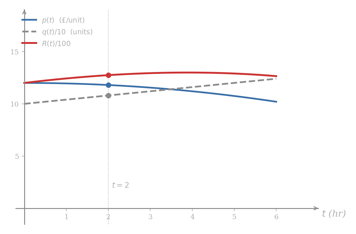
Three curves over the interval 0 ≤ t ≤ 6: the unit price p(t), the scaled inventory q(t)/10, and the scaled marked value R(t)/100 = p(t) q(t)/100. A vertical dotted line marks t = 2, where the slope of R(t)/100 is positive even though p(t) is decreasing.

The figure makes a structural point. The price curve $p(t)$ slopes down throughout the shift, yet the value curve $R(t)$ slopes up at $t = 2$ . Looking at $p$ alone or $q$ alone misses the answer. The product rule is what fuses the two contributions into a single rate.

Problem 106

A retailer’s sales volume $t$ weeks after launching a campaign is $V(t) = 200 + 30 t - t^2$ units per week, while the unit margin (profit per unit) is $m(t) = 5 + 0{.}1 \, t$ pounds. The total weekly profit is $\Pi(t) = m(t) \, V(t)$ .

Use the product rule to find $\Pi'(t)$ .
Compute $\Pi'(4)$ and explain in plain language whether weekly profit is rising or falling four weeks in, and at what rate, in pounds per week per week.
Find the time at which weekly profit is maximized on the interval $0 \leq t \leq 30$ .

Example 107 (Peak drug concentration)

A bolus injection produces a bloodstream concentration of

C(t) = (3 t + 1)^2 (2 - t), \qquad 0 \leq t \leq 2,

with $t$ measured in hours. Find the time at which $C$ peaks.

Set $f(t) = (3 t + 1)^2$ and $g(t) = 2 - t$ . Then $g'(t) = -1$ , and the general power rule gives $f'(t) = 2 (3 t + 1)(3) = 6 (3 t + 1)$ . By the product rule,

C'(t) = (3 t + 1)^2 (-1) + (2 - t) \cdot 6 (3 t + 1) = (3 t + 1)\bigl[-(3 t + 1) + 6 (2 - t)\bigr].

The bracket simplifies to $-3 t - 1 + 12 - 6 t = 11 - 9 t$ , so

C'(t) = (3 t + 1)(11 - 9 t).

Critical numbers come from $3 t + 1 = 0$ , giving $t = -1/3$ (outside the domain), and $11 - 9 t = 0$ , giving $t = 11/9 \approx 1{.}22$ . The endpoints contribute $C(0) = 2$ and $C(2) = 0$ , while

C\!\left(\tfrac{11}{9}\right) = \left(\tfrac{11}{3} + 1\right)^{\!2}\!\left(2 - \tfrac{11}{9}\right) = \left(\tfrac{14}{3}\right)^{\!2}\!\left(\tfrac{7}{9}\right) = \frac{196}{9} \cdot \frac{7}{9} = \frac{1372}{81} \approx 16{.}94.

The concentration peaks at $t = 11/9$ hours, well above either endpoint.

Concentration curve C(t) = (3t+1)² (2 - t) on [0, 2]. The curve starts at (0, 2), peaks near (11/9, 16.94) with dotted reference lines, and falls to (2, 0).

The factored form of $C'(t)$ also encodes the sign of the derivative directly: on $0 \leq t < 11/9$ both factors are positive so $C$ rises; past $11/9$ the second factor flips sign and $C$ falls. The first derivative test confirms the maximum without a separate sign chart.

Problem 107

A particle moves so that its position at time $t$ is $s(t) = (t^2 + 1)(t - 3)^2$ meters for $t \geq 0$ . The velocity is $v(t) = s'(t)$ .

Find $v(t)$ using the product rule and the general power rule, factoring fully.
Determine when the particle is momentarily at rest.
On which interval is the particle moving in the positive direction?

A Three-Factor Product

Applying the product rule twice handles three-factor products. Write $f \, g \, h = (f g) h$ and differentiate:

\frac{d}{dx}(f g h) = (f g) h' + h \cdot \frac{d}{dx}(f g) = f g \, h' + h (f g' + g f') = f' g h + f g' h + f g h'.

Each factor, in turn, gets differentiated while the other two are held; the three contributions are summed. The same pattern extends to any number of factors.

Example 108 (A three-factor product)

Differentiate $y = x \, (x - 2)(x^2 + 1)$ .

By the three-factor pattern with $f = x$ , $g = x - 2$ , $h = x^2 + 1$ :

\frac{dy}{dx} = (1)(x - 2)(x^2 + 1) + x(1)(x^2 + 1) + x(x - 2)(2 x).

Each term keeps two factors intact and replaces the third with its derivative.

For solving $\frac{dy}{dx} = 0$ , multiply out:

\frac{dy}{dx} = (x - 2)(x^2 + 1) + x(x^2 + 1) + 2 x^2 (x - 2) = (2 x - 2)(x^2 + 1) + 2 x^2 (x - 2).

Expanding gives $4 x^3 - 6 x^2 + 2 x - 2$ . The grouped form is more compact than expanding $y$ first into a degree-four polynomial and applying the power rule term by term, especially when one factor is itself a composite that the general power rule can absorb.

Problem 108

Differentiate $y = x^2 (x - 1)(x + 3)$ as a three-factor product. Then simplify, factor $y'$ over the integers as far as possible, and use the quadratic formula to list every $x$ for which $\dfrac{dy}{dx} = 0$ .

Problem 109

Let $y = f(x) \, g(x) \, h(x)$ where $f(2) = 3$ , $g(2) = -1$ , $h(2) = 4$ , $f'(2) = 5$ , $g'(2) = 2$ , $h'(2) = -3$ . Compute $\dfrac{dy}{dx}\bigg|_{x = 2}$ using the three-factor product rule.

Problem 110

Let $f_{1}, f_{2}, f_{3}, f_{4}$ be differentiable. Show that

\frac{d}{dx}\bigl[f_{1}(x) f_{2}(x) f_{3}(x) f_{4}(x)\bigr] = f_{1}' f_{2} f_{3} f_{4} + f_{1} f_{2}' f_{3} f_{4} + f_{1} f_{2} f_{3}' f_{4} + f_{1} f_{2} f_{3} f_{4}',

by applying the three-factor pattern from the A three-factor product example to $(f_{1} f_{2} f_{3}) \cdot f_{4}$ .

Then use the four-factor formula to compute $y'(0)$ for $y = (x - 1)(x - 2)(x - 3)(x - 4)$ — without expanding the polynomial — and verify directly by expanding $y$ and using the power rule.

Products are now handled. Ratios remain. The denominator in $G(x) = \dfrac{x^3}{(x^2 + 1)^4}$ from the opening can be moved upstairs as $(x^2 + 1)^{-4}$ and absorbed into a product, but the bookkeeping is fragile and the simplification messy. A direct rule for $f/g$ is cleaner and handles every applied ratio — cost per unit, density per area, return per pound invested, concentration per volume — without rewriting. The deeper payoff is structural: with a direct rule, the rate of change of an average has a clean relationship to the marginal, and that relationship falls out of the algebra automatically.

The Quotient Rule

Theorem 14 (Quotient Rule)

If $f$ and $g$ are differentiable at $x$ and $g(x) \neq 0$ , then $f/g$ is differentiable at $x$ , and

\frac{d}{dx} \!\left[ \frac{f(x)}{g(x)} \right] = \frac{g(x) \, f'(x) - f(x) \, g'(x)}{[g(x)]^2}.

The order of the two terms in the numerator matters: there is a minus sign between them. A standard mnemonic is “low d-high minus high d-low, square the bottom and away we go”: the denominator $g$ (“low”) times the derivative of the numerator $f$ (“d-high”), minus the numerator $f$ (“high”) times the derivative of the denominator $g$ (“d-low”), all over the denominator squared. Reversing the two products in the numerator changes the sign of the answer.

We postpone the proof until the rule has earned its keep through examples; the derivation appears later in this lesson, built directly on the product rule above together with the general power rule from Recitation 2.

Worked Quotient Examples

Example 109 (A first quotient)

Differentiate $y = \dfrac{x}{2 x + 3}$ .

Set $f(x) = x$ and $g(x) = 2 x + 3$ . Then $f'(x) = 1$ and $g'(x) = 2$ . By the quotient rule,

\frac{dy}{dx} = \frac{(2 x + 3)(1) - (x)(2)}{(2 x + 3)^2} = \frac{2 x + 3 - 2 x}{(2 x + 3)^2} = \frac{3}{(2 x + 3)^2}.

The cancellation in the numerator is the feature: even though both $f$ and $g$ contribute, their linear pieces meet so cleanly that the derivative reduces to a single constant over the squared denominator. That is the rule behaving well.

Problem 111

Differentiate each function using the quotient rule. Where simplification reveals critical numbers, leave the answer in fully factored form.

$y = \dfrac{2 x - 1}{x + 4}$ .
$y = \dfrac{x^2}{x^2 + 1}$ .
$y = \dfrac{x^2 + 1}{x^2 - 1}$ .
$y = \dfrac{(x + 2)^3}{x - 1}$ .

Example 110 (Simplifying after the quotient rule)

Find $\dfrac{dy}{dx}$ where $y = \dfrac{x^3}{(x^2 + 1)^4}$ .

Set $f(x) = x^3$ and $g(x) = (x^2 + 1)^4$ . Then $f'(x) = 3 x^2$ , and the general power rule gives $g'(x) = 4 (x^2 + 1)^3 (2 x) = 8 x (x^2 + 1)^3$ . The quotient rule supplies

\frac{dy}{dx} = \frac{(x^2 + 1)^4 \cdot 3 x^2 - x^3 \cdot 8 x (x^2 + 1)^3}{[(x^2 + 1)^4]^2} = \frac{(x^2 + 1)^4 \cdot 3 x^2 - 8 x^4 (x^2 + 1)^3}{(x^2 + 1)^8}.

Numerator and denominator share the factor $(x^2 + 1)^3$ . Cancelling it once,

\frac{dy}{dx} = \frac{(x^2 + 1)(3 x^2) - 8 x^4}{(x^2 + 1)^5} = \frac{3 x^4 + 3 x^2 - 8 x^4}{(x^2 + 1)^5} = \frac{x^2 (3 - 5 x^2)}{(x^2 + 1)^5}.

Critical numbers come from the numerator: $x = 0$ (a double root) or $5 x^2 = 3$ , giving $x = \pm \sqrt{3/5}$ . None of these would have been visible without the simplification.

Problem 112

Find $\dfrac{dy}{dx}$ where $y = \dfrac{x^2}{(x^2 + 4)^3}$ . Simplify the answer by cancelling the largest factor common to the entire numerator and denominator, and identify every $x$ at which $\dfrac{dy}{dx} = 0$ .

Remark

Cancelling here works because $(x^2 + 1)^3$ is a factor of the whole numerator and the whole denominator. A common term that appears as a summand — not as a factor — never cancels. The next example exists to make this crystal clear.

Example 111 (When nothing cancels)

Differentiate $y = \dfrac{x}{x + (x + 1)^3}$ .

Set $f(x) = x$ and $g(x) = x + (x + 1)^3$ . Then $f'(x) = 1$ , and by the sum rule and general power rule $g'(x) = 1 + 3 (x + 1)^2$ . The quotient rule gives

\frac{dy}{dx} = \frac{\bigl[x + (x + 1)^3\bigr](1) - x \bigl[1 + 3 (x + 1)^2\bigr]}{\bigl[x + (x + 1)^3\bigr]^2}.

Expanding the numerator:

\frac{dy}{dx} = \frac{x + (x + 1)^3 - x - 3 x (x + 1)^2}{\bigl[x + (x + 1)^3\bigr]^2} = \frac{(x + 1)^3 - 3 x (x + 1)^2}{\bigl[x + (x + 1)^3\bigr]^2}.

The numerator does have a clean factor of $(x + 1)^2$ :

\frac{dy}{dx} = \frac{(x + 1)^2 \bigl[(x + 1) - 3 x\bigr]}{\bigl[x + (x + 1)^3\bigr]^2} = \frac{(x + 1)^2 (1 - 2 x)}{\bigl[x + (x + 1)^3\bigr]^2}.

The denominator does not factor as $(x+1)^2 \cdot (\text{something})$ , even though $(x+1)^2$ shows up inside it after expansion: $x + (x+1)^3$ is a sum, not a product. A trainee instinct to “cancel the $(x+1)^2$ from top and bottom” would silently invent a wrong derivative. Cancellation is a property of factorizations, not of shared substrings.

Problem 113

Differentiate $y = \dfrac{(x + 1)^2}{x + (x - 1)^2}$ . Identify which factors do and do not cancel — recall the warning in the When nothing cancels example above — and simplify only as far as is justified.

Layered Rules

The quotient rule almost always cooperates with the product and general power rules. Decomposing the work cleanly is the only difficulty; the individual derivatives are routine.

Example 112 (A square root of a quotient)

Differentiate $f(x) = \sqrt{\dfrac{x^2 + 7}{x + 1}}$ .

On the real differentiable domain $x > -1$ , write $f$ as a power: $f(x) = \!\left(\dfrac{x^2 + 7}{x + 1}\right)^{\!1/2}$ . The general power rule with $r = 1/2$ gives

f'(x) = \frac{1}{2} \!\left(\frac{x^2 + 7}{x + 1}\right)^{\!-1/2} \frac{d}{dx} \!\left[\frac{x^2 + 7}{x + 1}\right]. \tag{3}

The inner derivative is the genuine quotient computation. Set $u(x) = x^2 + 7$ and $v(x) = x + 1$ . Then $u' = 2 x$ and $v' = 1$ , so

\frac{d}{dx} \!\left[\frac{x^2 + 7}{x + 1}\right] = \frac{(x + 1)(2 x) - (x^2 + 7)(1)}{(x + 1)^2} = \frac{x^2 + 2 x - 7}{(x + 1)^2}.

Substituting back into $(3)$ :

f'(x) = \frac{1}{2} \!\left(\frac{x^2 + 7}{x + 1}\right)^{\!-1/2} \frac{x^2 + 2 x - 7}{(x + 1)^2}.

To simplify, use $\!\left(\dfrac{a}{b}\right)^{\!-1/2} = \!\left(\dfrac{b}{a}\right)^{\!1/2}$ :

f'(x) = \frac{1}{2} \!\left(\frac{x + 1}{x^2 + 7}\right)^{\!1/2} \frac{x^2 + 2 x - 7}{(x + 1)^2} = \frac{1}{2} \cdot \frac{(x + 1)^{1/2}}{(x^2 + 7)^{1/2}} \cdot \frac{x^2 + 2 x - 7}{(x + 1)^2}.

Combining the factors of $(x + 1)$ :

f'(x) = \frac{x^2 + 2 x - 7}{2 (x^2 + 7)^{1/2} (x + 1)^{3/2}}.

The full computation took three rules layered: the general power rule on the outside, the quotient rule on the inside, and elementary exponent identities to put the answer in standard form. The architecture — outer rule first, inner pieces afterwards — is the same for every nested differentiation problem in this course.

Problem 114

Differentiate $f(x) = \sqrt{\dfrac{x + 1}{x^2 + 1}}$ by writing $f$ as a power and combining the general power rule with the quotient rule. State $f'(x)$ with no negative exponents, writing fractional powers as square roots.

Problem 115

The tangent line to the curve $y = \sqrt{x^{2} + 9}$ at the point with $x = 4$ is the line $y = mx + b$ for unique constants $m$ and $b$ .

Use the general power rule and the chain rule to compute $m$ , then find $b$ from the point-slope form.
Show that the equation $\sqrt{x^{2} + 9} = mx + b$ — equating the curve to its tangent line — has $x = 4$ as a double root by squaring both sides and reducing to a polynomial. (A simple root would mean the tangent crosses the curve transversally; a double root reflects the tangent’s first-order contact with the curve.)
State, in one sentence, why a double root at $x = 4$ is the algebraic version of the geometric fact that the tangent line touches the curve there.

At a Minimum, Average Cost Equals Marginal Cost

The quotient rule’s most repeated economic application is to averages. Average cost is, by definition, the ratio of total cost to output. Marginal cost is the derivative of total cost. The quotient rule produces a precise relationship between the two at the optimum.

Example 113 (Average cost meets marginal cost)

Suppose the total cost of producing $x$ units is $C(x)$ . Define the average cost per unit $AC(x) = C(x)/x$ and the marginal cost $MC(x) = C'(x)$ . Show that, at any positive output level where $AC$ has a local minimum, the equality $AC = MC$ holds.

Differentiate $AC$ using the quotient rule with $f(x) = C(x)$ and $g(x) = x$ :

\frac{d}{dx} (AC) = \frac{x \cdot C'(x) - C(x) \cdot 1}{x^2} = \frac{x \, C'(x) - C(x)}{x^2}.

At such a minimum of $AC$ , we must have $\dfrac{d}{dx}(AC) = 0$ . With $x > 0$ the denominator $x^2$ is positive, so the equation reduces to

x \, C'(x) - C(x) = 0.

Adding $C(x)$ to both sides and then dividing by $x$ gives

C'(x) = \frac{C(x)}{x},

that is, $MC(x) = AC(x)$ .

The two cost curves cross at any positive output where the average cost is minimized.

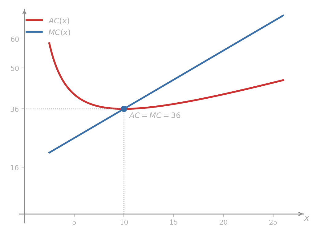
Average cost AC(x) = x + 16 + 100/x and marginal cost MC(x) = 2x + 16 plotted on the same axes. AC is U-shaped with minimum at x = 10; MC is a rising line that crosses AC exactly at the minimum, with both curves equal to 36 there.

The figure makes the geometry concrete. With $C(x) = x^2 + 16 x + 100$ , the average cost $AC(x) = x + 16 + 100/x$ is the structurally familiar curve of Lesson 3PM (a linear term plus a reciprocal term, single minimum at $x = 10$ , where $AC = 36$ ). The marginal cost $MC(x) = 2 x + 16$ is a straight line with slope $2$ , hitting $36$ exactly at $x = 10$ . The intersection point and the minimum point coincide.

The economic reading is immediate: while the cost of producing the next unit is below the average, additional production pulls the average down; when the next unit costs more than the average, additional production pushes the average up. Equality is the fixed point.

Problem 116

A factory’s daily total cost in pounds, when producing $x$ units per day, is

C(x) = 0{.}5 \, x^2 + 30 \, x + 200.

Write $AC(x)$ and $MC(x)$ .
Use the quotient rule to find $AC'(x)$ and the production level minimizing $AC$ .
Verify directly that $AC = MC$ at the optimum, in line with the Average cost meets marginal cost result.

Problem 117

The result $AC = MC$ at a positive-output minimum of $AC$ used only that $AC = C/x$ and that $x > 0$ . Adapt the argument to show that, for any differentiable function $h(x) = u(x)/x$ with $x > 0$ , every relative extremum of $h$ occurs where $u'(x) = u(x)/x$ . State, in plain English, what this says about averages of any non-negative quantity that varies with $x$ .

A Quotient Optimization

Example 114 (Maximizing return on investment)

A small firm’s monthly return on each pound invested, $t$ months after the initial outlay, is modeled by

R(t) = \frac{50 \, t}{t^2 + 25}, \qquad t \geq 0,

in pence per pound (i.e. units of $1/100$ pound). Find the time at which the return is highest.

Set $f(t) = 50 \, t$ and $g(t) = t^2 + 25$ , so $f'(t) = 50$ and $g'(t) = 2 t$ . By the quotient rule,

R'(t) = \frac{(t^2 + 25)(50) - (50 \, t)(2 t)}{(t^2 + 25)^2} = \frac{50 \, t^2 + 1250 - 100 \, t^2}{(t^2 + 25)^2} = \frac{50 \, (25 - t^2)}{(t^2 + 25)^2}.

The denominator is positive for every $t$ , so the sign of $R'(t)$ is determined by $25 - t^2$ . Setting $R'(t) = 0$ gives $t^2 = 25$ , so $t = 5$ (the negative root is outside the domain). For $0 \leq t < 5$ , $25 - t^2 > 0$ and $R$ is increasing; for $t > 5$ , $R$ is decreasing. By the first derivative test, $t = 5$ is the absolute maximum on $[0, \infty)$ .

The peak return is

R(5) = \frac{50 \cdot 5}{25 + 25} = \frac{250}{50} = 5.

The investment yields its highest monthly return — 5 pence per pound — exactly five months after the outlay.

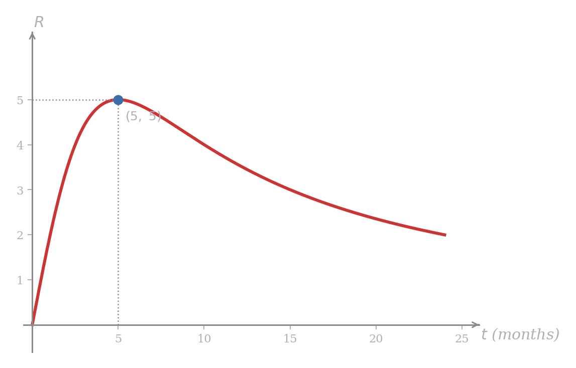
Curve R(t) = 50t/(t² + 25) on the displayed interval. The curve rises sharply from the origin, peaks at (5, 5) with dotted reference lines, and decays slowly afterwards as the denominator grows faster than the numerator.

The shape has a structural lesson. For small positive $t$ , the linear numerator $50 \, t$ outpaces the denominator $t^2 + 25$ (which is dominated by its constant $25$ ). For large $t$ , the denominator’s quadratic term takes over and the ratio decays like $50/t$ . In this model, those two effects balance at one peak, and the quotient rule locates it.

Problem 118

Pollutant concentration in a tank, $t$ minutes after a spill, is modeled by

P(t) = \frac{60 \, t}{t^2 + 9} \text{ ppm}, \qquad t \geq 0.

Find $P'(t)$ using the quotient rule and factor it.
Determine the time at which concentration peaks and the peak value.
The clean-up team must intervene before $P$ exceeds $9$ ppm. Has the peak been reached at the moment $P$ first hits $9$ ppm, or is it still rising?

Problem 119

A daily delivery service models its profit per kilometer driven by

\Pi(d) = \frac{40 \, d - d^2}{d + 5}, \qquad 0 \leq d \leq 40,

in pounds per kilometer.

Use the quotient rule to find $\Pi'(d)$ and simplify.
Find every critical number on the open interval and classify each.
Compare each critical value with the endpoint values and identify the absolute maximum.

Proof of the Quotient Rule

The quotient rule does not need its own limit-definition argument. It follows from the product rule above and the general power rule applied to $[g(x)]^{-1}$ .

Proof

Step 1: a reciprocal derivative. The general power rule from Recitation 2 extends to negative integer exponents. Since $g(x) \neq 0$ and $g$ is continuous at $x$ , the reciprocal is defined for inputs near $x$ . With $r = -1$ ,

\frac{d}{dx} \!\left[\frac{1}{g(x)}\right] = \frac{d}{dx} [g(x)]^{-1} = (-1) [g(x)]^{-2} \cdot g'(x) = -\frac{g'(x)}{[g(x)]^2}.

Step 2: write the quotient as a product and apply the product rule. For $g(x) \neq 0$ ,

\frac{f(x)}{g(x)} = f(x) \cdot \frac{1}{g(x)},

so by the product rule,

\frac{d}{dx} \!\left[\frac{f(x)}{g(x)}\right] = \frac{1}{g(x)} \cdot f'(x) + f(x) \cdot \frac{d}{dx} \!\left[\frac{1}{g(x)}\right].

Substituting Step 1:

\frac{d}{dx} \!\left[\frac{f(x)}{g(x)}\right] = \frac{f'(x)}{g(x)} - \frac{f(x) \, g'(x)}{[g(x)]^2} = \frac{g(x) \, f'(x)}{[g(x)]^2} - \frac{f(x) \, g'(x)}{[g(x)]^2} = \frac{g(x) \, f'(x) - f(x) \, g'(x)}{[g(x)]^2}.

■

The minus sign in the numerator now has a clear origin: it tracks back to the $(-1)$ exponent in $[g(x)]^{-1}$ , which is the only minus sign in the entire chain of substitutions. Forgetting the minus sign in the rule is forgetting that one is differentiating the reciprocal, not multiplying by it.

Problem 120

Use the reciprocal-derivative formula from Step 1 of the proof above to differentiate

y = \frac{1}{(x^3 - 2 x + 5)^2}

in two ways: first by writing $y$ as $[g(x)]^{-2}$ and applying the general power rule directly, second by writing $y$ as $1 / [g(x)]^2$ and applying the quotient rule. Confirm that the two answers agree.

Quotients are now handled. The remaining structural gap from the opening is composition: an outer function $f$ applied to an inner function $g$ , written $f(g(x))$ . The general power rule above is the special case where the outer function is a power, $f(x) = x^r$ ; for example, $H(x) = \sqrt{4 x^2 + 1}$ is already covered by taking $r = 1/2$ . The chain rule is the same idea generalized: any differentiable outer function applied to any differentiable inner function gets a clean derivative.

Composition

Two functions $f$ and $g$ compose into a third by feeding the output of $g$ into the input of $f$ .

Definition 34 (Composition)

Given functions $f$ and $g$ , the composition $f \circ g$ is the function defined by

(f \circ g)(x) = f(g(x)),

on the set of $x$ for which $g(x)$ lies in the domain of $f$ . We call $f$ the outside function and $g$ the inside function.

Recognizing a function as a composite is half the work; the chain rule then differentiates it mechanically.

Example 115 (Building a composition)

Let $f(x) = \dfrac{x - 1}{x + 1}$ and $g(x) = x^3$ . Then

f(g(x)) = \frac{g(x) - 1}{g(x) + 1} = \frac{x^3 - 1}{x^3 + 1}.

Each occurrence of $x$ in $f(x)$ is replaced by $g(x)$ .

Example 116 (Decomposing into outer and inner pieces)

Identify each function as $f(g(x))$ and name the outer and inner pieces.

$h(x) = (x^5 + 9 x + 3)^8$ . Outside: $f(x) = x^8$ . Inside: $g(x) = x^5 + 9 x + 3$ .
$k(x) = \sqrt{4 x^2 + 1}$ . Outside: $f(x) = \sqrt{x}$ . Inside: $g(x) = 4 x^2 + 1$ .

The decomposition is rarely unique — $h$ above can also be read as $(x^5 + 9 x + 3)^4$ to the power $2$ , with $f(x) = x^2$ — but every decomposition leads to the same derivative when the chain rule is applied.

A function of the form $[g(x)]^r$ is the composite $f(g(x))$ with outside $f(x) = x^r$ . The general power rule already gave its derivative,

\frac{d}{dx} [g(x)]^r = r [g(x)]^{r-1} \, g'(x),

and the chain rule has the same shape, with $f$ free to be anything differentiable.

The Chain Rule

Theorem 15 (Chain Rule)

If $g$ is differentiable at $x$ and $f$ is differentiable at $g(x)$ , then $f \circ g$ is differentiable at $x$ , and

\frac{d}{dx} f(g(x)) = f'(g(x)) \cdot g'(x).

In words: differentiate the outside, leave the inside alone, then multiply by the derivative of the inside.

The two factors play different roles. $f'(g(x))$ asks how fast the outside function is changing at the value the inside has just produced; $g'(x)$ asks how fast the inside function is changing at $x$ . The product is the rate of change of the composition.

Example 117 (The general power rule recovered)

Use the chain rule on $f(g(x))$ with $f(x) = x^8$ and $g(x) = x^5 + 9 x + 3$ .

We have $f'(x) = 8 x^7$ and $g'(x) = 5 x^4 + 9$ , so

f'(g(x)) = 8 (x^5 + 9 x + 3)^7,

and the chain rule gives

\frac{d}{dx} f(g(x)) = 8 (x^5 + 9 x + 3)^7 (5 x^4 + 9).

The outside is a power, so the answer matches what the general power rule produces directly. The chain rule does not change the answer; it labels the structure of the calculation in a way that survives when the outside is no longer a power.

Example 118 (Differentiating an unspecified outer function)

Let $h(x) = f(\sqrt{x})$ for some differentiable $f$ (no formula given). Find $h'(x)$ in terms of $f'$ .

Set $g(x) = \sqrt{x}$ , so $h = f \circ g$ . The general power rule gives $g'(x) = \dfrac{1}{2 \sqrt{x}}$ , and the chain rule supplies

h'(x) = f'(g(x)) \cdot g'(x) = f'(\sqrt{x}) \cdot \frac{1}{2 \sqrt{x}} = \frac{f'(\sqrt{x})}{2 \sqrt{x}}.

The outside function is opaque, yet the chain rule still tells us exactly how the rate of change of $h$ depends on the rate of change of $f$ . This pattern — passing through an unknown outer function — is the central maneuver when implicit and inverse functions enter the course.

Problem 121

Let $h(x) = f(x^2 + 1)$ where $f$ is differentiable.

Express $h'(x)$ in terms of $f'$ .
Given $f'(5) = 7$ , compute $h'(2)$ .

Problem 122

Let $F(x) = \bigl[ g(x) \bigr]^3$ where $g(2) = -1$ and $g'(2) = 4$ . Use the chain rule to compute $F'(2)$ .

Problem 123

For each function, identify the outside $f$ and the inside $g$ , then differentiate using the chain rule.

$h(x) = (3 x^2 - 5)^7$ .
$h(x) = \sqrt{x^3 + x + 1}$ .
$h(x) = \dfrac{1}{(x^2 + 4)^3}$ .
$h(x) = \bigl( (2 x + 1)^4 + 7 \bigr)^{1/2}$ (a chain of two compositions; treat the inner composite as $g$ ).

Leibniz Form

Setting $u = g(x)$ and $y = f(u)$ converts the chain rule into a notation that mirrors how rates compose physically. Then $\dfrac{du}{dx} = g'(x)$ and $\dfrac{dy}{du} = f'(u) = f'(g(x))$ , and the chain rule becomes

\frac{dy}{dx} = \frac{dy}{du} \cdot \frac{du}{dx}. \tag{4}

The derivative symbols are not literal fractions, but the apparent cancellation of the $du$ symbols is a faithful mnemonic.

The interpretation is direct. If $y$ varies three times as fast as $u$ and $u$ varies twice as fast as $x$ , then $y$ varies six times as fast as $x$ :

\frac{dy}{dx} = 3 \cdot 2 = 6.

Rates compose by multiplication, just as scaling factors do.

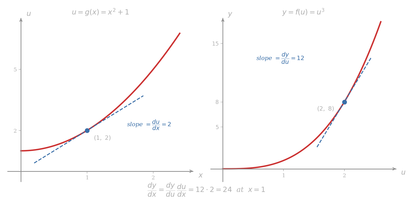
Two graphs side by side. Left: u = x² + 1 with the tangent at x = 1 marked, slope du/dx = 2. Right: y = u³ with the tangent at u = 2 marked, slope dy/du = 12. The composition gives dy/dx = 12 × 2 = 24 at x = 1.

The figure makes the rule visible. With $u = x^2 + 1$ , at $x = 1$ we have $u = 2$ and $du/dx = 2$ . With $y = u^3$ , at $u = 2$ we have $y = 8$ and $dy/du = 12$ . The chain rule says $dy/dx = 12 \cdot 2 = 24$ at $x = 1$ , and substituting the composition $y = (x^2 + 1)^3$ confirms it: $\dfrac{dy}{dx} = 3 (x^2 + 1)^2 (2 x) = 6 x (x^2 + 1)^2 = 6 \cdot 1 \cdot 4 = 24$ at $x = 1$ .

Example 119 (The chain rule via

u

)

Find $\dfrac{dy}{dx}$ if $y = u^5 - 2 u^3 + 8$ and $u = x^2 + 1$ .

The relation $y(x)$ is not given directly. Differentiate $y$ with respect to $u$ and $u$ with respect to $x$ :

\frac{dy}{du} = 5 u^4 - 6 u^2, \qquad \frac{du}{dx} = 2 x.

By $(4)$ ,

\frac{dy}{dx} = (5 u^4 - 6 u^2) \cdot 2 x.

Expressing in $x$ alone via $u = x^2 + 1$ :

\frac{dy}{dx} = \bigl[ 5 (x^2 + 1)^4 - 6 (x^2 + 1)^2 \bigr] \cdot 2 x.

Substituting $u$ into $y$ first and then differentiating using only the rules above gives the same answer; it is just a longer calculation. The Leibniz form is preferred because the next two examples — and most of the applied work in later lessons — present the variables in exactly the layered way that $(4)$ exploits.

Problem 124

Find $\dfrac{dy}{dx}$ in two ways: first by substituting and differentiating directly, second by the chain rule via $u$ . Confirm the answers agree.

$y = u^4 + u^2$ , $u = 2 x + 3$ .
$y = \sqrt{u}$ , $u = x^2 + 7$ .
$y = \dfrac{1}{u}$ , $u = x^3 + x$ .

Problem 125

Suppose $y = f(u)$ , $u = g(v)$ , $v = h(x)$ , so that $y$ depends on $x$ through two compositions. Show that

\frac{dy}{dx} = \frac{dy}{du} \cdot \frac{du}{dv} \cdot \frac{dv}{dx},

by applying the two-link chain rule twice. Use this three-link form to differentiate $y = \sqrt{(3 x - 2)^6 + 5}$ .

Time Rates of Change

The chain rule’s most repeated applied use is to convert a rate of change with respect to one variable into a rate of change with respect to time. If $x$ is a function of $t$ and $R$ is a function of $x$ , then $R$ is a function of $t$ , and

\frac{dR}{dt} = \frac{dR}{dx} \cdot \frac{dx}{dt}.

The factor $\dfrac{dR}{dx}$ is the marginal quantity already studied in Lessons 2 and 3; the factor $\dfrac{dx}{dt}$ is how fast the input is moving in real time. Their product is the real-time rate of change of $R$ .

Example 120 (Marginal revenue and time)

A shop sells ties for £12 each. Let $x$ be the cumulative number of ties sold by time $t$ , and let $R = 12 x$ be the corresponding revenue. If sales are rising at four ties per day, how fast is revenue rising?

Each extra tie brings in £12, and four extras a day brings in £48 a day; the answer is intuitively £48 per day. The chain rule reproduces it:

\frac{dR}{dt} = \frac{dR}{dx} \cdot \frac{dx}{dt} = 12 \cdot 4 = 48 \text{ pounds per day}.

The factor $\dfrac{dR}{dx} = 12$ is the marginal revenue per tie; $\dfrac{dx}{dt} = 4$ is the sales rate in ties per day. The chain rule asserts that the time rate of revenue is always the product of these two — the marginal multiplied by the time rate of the input.

Example 121 (Time rate of revenue at a production target)

The demand equation for a brand of graphing calculator is $p = 86 - 0{.}002 \, x$ pounds per unit, where $x$ is the cumulative number of calculators produced and sold during the current run. The firm is currently at $x = 6000$ and is increasing production by $200$ calculators per day. Find the time rate of change of total revenue at this production level.

Total revenue is

R(x) = x \cdot p = x (86 - 0{.}002 \, x) = -0{.}002 \, x^2 + 86 \, x.

The marginal revenue is

\frac{dR}{dx} = -0{.}004 \, x + 86.

By the chain rule,

\frac{dR}{dt} = \frac{dR}{dx} \cdot \frac{dx}{dt} = (-0{.}004 \, x + 86) \cdot \frac{dx}{dt}.

At $x = 6000$ and $\dfrac{dx}{dt} = 200$ :

\frac{dR}{dt} = \bigl(-0{.}004 (6000) + 86\bigr) \cdot 200 = (-24 + 86) \cdot 200 = 62 \cdot 200 = 12\,400.

Revenue is rising at £12,400 per day at this production level.

Revenue parabola R(x) = -0.002x² + 86x for x in [0, 43000], with R rescaled by 1/1000. The current production point at x = 6000 is marked, with R = £444,000 and a tangent line of slope dR/dx = 62 (£ per unit).

The figure isolates the two factors visually. The slope of the tangent line at $x = 6000$ is $\dfrac{dR}{dx} = 62$ pounds per unit. That number is fixed by the demand model and the current production level; it has nothing to do with time. Plugging in $\dfrac{dx}{dt} = 200$ — the production schedule — converts that marginal into a daily rate. Different schedules yield different time rates while leaving the marginal unchanged: doubling the production speed to $400$ per day would double the time rate of revenue to £24,800 per day.

Example 122 (A balloon inflating)

Air is being pumped into a spherical balloon, and the radius is observed to grow at $\dfrac{dr}{dt} = 0{.}5$ centimeters per second when $r = 4$ centimeters. How fast is the volume changing at that instant?

The volume of a sphere is $V = \dfrac{4}{3} \pi r^3$ . Differentiating with respect to $r$ ,

\frac{dV}{dr} = 4 \pi r^2.

By the chain rule,

\frac{dV}{dt} = \frac{dV}{dr} \cdot \frac{dr}{dt} = 4 \pi r^2 \cdot \frac{dr}{dt}.

At $r = 4$ and $\dfrac{dr}{dt} = 0{.}5$ :

\frac{dV}{dt} = 4 \pi (16)(0{.}5) = 32 \pi \approx 100{.}5 \text{ cm}^3/\text{s}.

The factor $4 \pi r^2$ is the surface area of the sphere — geometrically, the rate at which volume changes per unit increase in radius is the area of the boundary. The chain rule turns that geometric fact into a time rate.

Problem 126

A circular oil slick is spreading. Its radius grows at $\dfrac{dr}{dt} = 2$ meters per minute when $r = 50$ meters. The slick’s area is $A = \pi r^2$ .

Write $\dfrac{dA}{dt}$ using the chain rule.
Compute $\dfrac{dA}{dt}$ at the moment $r = 50$ .
The slick’s circumference is $C = 2 \pi r$ . Find $\dfrac{dC}{dt}$ at the same instant. Why does the circumference rate not depend on the current value of $r$ ?

Problem 127

A factory’s daily revenue at production level $x$ is $R(x) = 200 x - 0{.}01 \, x^2$ pounds per day. The production schedule is $x(t) = 500 + 30 t$ units per day, where $t$ is in days from the start of the schedule.

Compute $\dfrac{dR}{dx}$ as a function of $x$ , and state the marginal revenue at $x = 500$ and at $x = 1000$ .
Use the chain rule to find $\dfrac{dR}{dt}$ .
At what value of $t$ does the time rate of daily revenue equal zero? Interpret what this means in plain English.

Problem 128

A spherical raindrop evaporates so that its radius decreases at $\dfrac{dr}{dt} = -0{.}02$ millimeters per second when $r = 1$ millimeter. Find $\dfrac{dV}{dt}$ at that instant, with $V = \dfrac{4}{3} \pi r^3$ . Why is the rate negative?

Problem 129

Two ships leave the same harbor at $t = 0$ . Ship $A$ travels due east at $30$ km/h; ship $B$ travels due north at $40$ km/h. Let $a(t)$ and $b(t)$ denote their distances from the harbor at time $t$ , and let $D(t) = \sqrt{a(t)^{2} + b(t)^{2}}$ denote the distance between the two ships.

Use the chain rule on $D = \sqrt{a^{2} + b^{2}}$ to express $\dfrac{dD}{dt}$ in terms of $a$ , $b$ , $\dfrac{da}{dt}$ , and $\dfrac{db}{dt}$ .
Compute $\dfrac{dD}{dt}$ at $t = 1$ hour. Then compute it again at $t = 2$ hours. Show the answers are equal.
Prove that $\dfrac{dD}{dt}$ is constant for every $t > 0$ , and explain in one sentence why the constancy is forced by the geometry of two perpendicular constant-speed motions.

Proof of the Chain Rule

The chain rule does not follow from earlier rules the way the quotient rule did. It needs its own limit argument, built around the trick of relating the difference quotient of $f \circ g$ at $x = a$ to the difference quotient of $f$ at $g(a)$ .

Proof

Suppose $g$ is differentiable at $a$ and $f$ is differentiable at $g(a)$ . Set $b = g(a)$ . Since $f$ is differentiable at $b$ , its change near $b$ can be written as

f(b+k)-f(b)=\bigl(f'(b)+E(k)\bigr)k,

where $E(k)$ tends to $0$ as $k$ tends to $0$ . For $k \neq 0$ , this is just the difference quotient rewritten:

E(k)=\frac{f(b+k)-f(b)}{k}-f'(b),

and at $k=0$ we may set $E(0)=0$ , so the displayed change formula remains true.

Now put $k = g(a+h)-g(a)$ . Since $g$ is differentiable at $a$ , it is continuous at $a$ , so this $k$ tends to $0$ as $h$ tends to $0$ . Also $g(a+h)=b+k$ . Therefore

f(g(a+h))-f(g(a)) = \bigl(f'(b)+E(g(a+h)-g(a))\bigr)\bigl(g(a+h)-g(a)\bigr).

Divide by $h$ :

\frac{f(g(a+h))-f(g(a))}{h} = \bigl(f'(b)+E(g(a+h)-g(a))\bigr)\frac{g(a+h)-g(a)}{h}.

Taking the limit as $h$ tends to $0$ , the first factor tends to $f'(b)$ and the second factor tends to $g'(a)$ . Hence

\left. \frac{d}{dx} f(g(x)) \right|_{x=a} = f'(b)g'(a) = f'(g(a))g'(a),

which is the chain rule at $x=a$ .

■

The proof’s central trick is the same one that powered the product rule: a single difference quotient is too tangled to evaluate, so we rewrite it using a bridge term whose limit we understand. For the product rule, the bridge term was $f(x + h) g(x)$ ; for the chain rule, the bridge is the inner change $g(a + h) - g(a)$ .

Note (Differentiation toolkit so far)

Combining the rules from Lessons 2, Recitation 2, and this lesson, every differentiable expression in this course can be reduced. Apply the rules from the outside in.

Rule	Form
Constant multiple	$\frac{d}{dx}[c \, f] = c \, f'$
Sum	$\frac{d}{dx}[f \pm g] = f' \pm g'$
Power	$\frac{d}{dx} x^n = n \, x^{n-1}$
Product	$\frac{d}{dx}[f \, g] = f \, g' + g \, f'$
Quotient	$\frac{d}{dx}\!\left[\frac{f}{g}\right] = \frac{g \, f' - f \, g'}{g^2}$
Chain	$\frac{d}{dx} f(g(x)) = f'(g(x)) \, g'(x)$
General power (chain ∘ power)	$\frac{d}{dx} [g(x)]^r = r \, [g(x)]^{r-1} g'(x)$

The general power rule is now formally what it always was structurally: the chain rule with $f(x) = x^r$ .