23/03/2026

#Math#Vectors#Geometry

Video

Lesson assets

video link

CS50P Lecture 0: Functions, Variables

recitation

Lesson 3 Recitation

homework

Homework 3 PDF

Matrices

The general $m \times n$ system written out at the end of Lesson 3AM already arranges its coefficients $a_{ij}$ in $m$ rows and $n$ columns on the page, and its right-hand sides $b_i$ in a single column of length $m$ . Up to now those two rectangles were only typographic scaffolding for the equations. Once they are named as objects of their own, every question about existence, uniqueness, and structure of the system becomes a question about them, and the individual unknowns $x_j$ drop out of the bookkeeping. The rest of the course is essentially the study of those rectangles.

The Rectangular Array

Definition 36 (Rectangular Matrix)

An $m \times n$ matrix over a field $\mathbb{F}$ is an ordered array of $mn$ scalars $a_{ij} \in \mathbb{F}$ , indexed by $1 \le i \le m$ and $1 \le j \le n$ , arranged in $m$ rows and $n$ columns:

A = \begin{bmatrix} a_{11} & a_{12} & \cdots & a_{1n} \\ a_{21} & a_{22} & \cdots & a_{2n} \\ \vdots & \vdots & & \vdots \\ a_{m1} & a_{m2} & \cdots & a_{mn} \end{bmatrix}.

The scalar $a_{ij}$ is the entry of $A$ at row $i$ and column $j$ , and the pair $(m, n)$ is the size of $A$ . We shorten the display to

A = [a_{ij}]_{i,\, j = 1}^{m,\, n}, \qquad \text{or} \qquad A = [a_{ij}]

when the index ranges are clear from context. The set of all $m \times n$ matrices over $\mathbb{F}$ is written $\mathbb{F}^{m \times n}$ ; in particular, when $\mathbb{F} = \mathbb{R}$ we write $\mathbb{R}^{m \times n}$ .

The field $\mathbb{F}$ is the generic field introduced at the close of Lesson 3AM; unless stated otherwise the default reading $\mathbb{F} = \mathbb{R}$ remains in force.

Definition 37 (Equality of Matrices)

Matrices $A = [a_{ij}]$ and $B = [b_{ij}]$ are equal, written $A = B$ , if and only if they have the same size $(m, n)$ and $a_{ij} = b_{ij}$ for every $1 \le i \le m$ and $1 \le j \le n$ .

The size requirement is not redundant. A $2 \times 3$ and a $3 \times 2$ matrix with the same multiset of entries are never equal, because the index pairs on either side of the proposed equality do not even match up.

Example 47 (The Coefficient Matrix of a System)

The system at the end of Lesson 3AM,

\begin{cases} x + y + z = 1, \\ x - y + 2z = 0, \end{cases}

has $m = 2$ equations in $n = 3$ unknowns, so its coefficient table is the $2 \times 3$ matrix

A = \begin{bmatrix} 1 & 1 & 1 \\ 1 & -1 & 2 \end{bmatrix} \in \mathbb{R}^{2 \times 3},

while its right-hand sides form the $2 \times 1$ column

\mathbf{b} = \begin{bmatrix} 1 \\ 0 \end{bmatrix} \in \mathbb{R}^{2 \times 1}.

The pair $(A, \mathbf{b})$ determines the system: the unknowns $x, y, z$ never appear once the entries have been read off. Row reduction and every later test for existence, uniqueness, and structure will be carried out on $(A, \mathbf{b})$ without rewriting the equations.

Square Matrices and Diagonals

The coefficient matrix of a system is square precisely when the number of equations equals the number of unknowns, the case where geometric intuition in $\mathbb{R}^2$ and $\mathbb{R}^3$ from the two earlier lessons was sharpest: two non-parallel lines meeting in a point, three generic planes meeting in a point. A dedicated vocabulary for the square case is worth pinning down before we have to exercise it.

Definition 38 (Square Matrix and Its Diagonals)

A matrix $A = [a_{ij}] \in \mathbb{F}^{n \times n}$ is square, and its common side length $n$ is the order of $A$ . The entries $a_{11}, a_{22}, \ldots, a_{nn}$ form the main diagonal of $A$ ; the entries $a_{1n}, a_{2,\, n-1}, \ldots, a_{n1}$ form the secondary diagonal:

A = \begin{bmatrix} \color{#c0392b}{a_{11}} & a_{12} & \cdots & \color{#2874a6}{a_{1n}} \\ a_{21} & \color{#c0392b}{a_{22}} & \cdots & a_{2n} \\ \vdots & \vdots & \ddots & \vdots \\ \color{#2874a6}{a_{n1}} & a_{n2} & \cdots & \color{#c0392b}{a_{nn}} \end{bmatrix},

with the main diagonal picked out in red and the secondary diagonal in blue.

The main diagonal is where self-interaction sits: in a square system the coefficient $a_{ii}$ measures how strongly the $i$ th equation depends on the $i$ th unknown, and the structure of the remainder governs how quickly an elimination schedule can clean that dependence up.

Triangular and Diagonal Matrices

The square systems easiest to solve by hand are those whose coefficient matrix already has half of its off-diagonal entries equal to zero.

Definition 39 (Triangular Matrix)

A square matrix $A = [a_{ij}] \in \mathbb{F}^{n \times n}$ is upper triangular when $a_{ij} = 0$ for every $i > j$ , and lower triangular when $a_{ij} = 0$ for every $i < j$ . Schematically,

A_{\text{upper}} = \begin{bmatrix} a_{11} & a_{12} & \cdots & a_{1n} \\ 0 & a_{22} & \cdots & a_{2n} \\ \vdots & & \ddots & \vdots \\ 0 & \cdots & 0 & a_{nn} \end{bmatrix}, \qquad A_{\text{lower}} = \begin{bmatrix} a_{11} & 0 & \cdots & 0 \\ a_{21} & a_{22} & \cdots & 0 \\ \vdots & \vdots & \ddots & \vdots \\ a_{n1} & a_{n2} & \cdots & a_{nn} \end{bmatrix}.

An upper triangular system is solved by back-substitution: the last row fixes $x_n$ , the penultimate row fixes $x_{n-1}$ once $x_n$ is known, and so on up. Lower triangular systems are solved the same way from the top down. The whole apparatus of row reduction, developed from the next lesson on, aims at one of these two shapes.

Definition 40 (Diagonal, Scalar, Identity, and Zero Matrices)

A square matrix $A = [a_{ij}] \in \mathbb{F}^{n \times n}$ is diagonal when $a_{ij} = 0$ for every $i \neq j$ ; equivalently, when it is both upper and lower triangular:

\operatorname{diag}(a_{11}, a_{22}, \ldots, a_{nn}) = \begin{bmatrix} a_{11} & 0 & \cdots & 0 \\ 0 & a_{22} & \cdots & 0 \\ \vdots & \vdots & \ddots & \vdots \\ 0 & 0 & \cdots & a_{nn} \end{bmatrix}.

When all those diagonal entries are the same scalar $a \in \mathbb{F}$ , the matrix is scalar; the case $a = 1$ is the identity matrix $I$ , and the case $a = 0$ is the square zero matrix $\mathbf{0}$ :

aI = \begin{bmatrix} a & 0 & \cdots & 0 \\ 0 & a & \cdots & 0 \\ \vdots & \vdots & \ddots & \vdots \\ 0 & 0 & \cdots & a \end{bmatrix}, \qquad I = \begin{bmatrix} 1 & 0 & \cdots & 0 \\ 0 & 1 & \cdots & 0 \\ \vdots & \vdots & \ddots & \vdots \\ 0 & 0 & \cdots & 1 \end{bmatrix}, \qquad \mathbf{0} = \begin{bmatrix} 0 & 0 & \cdots & 0 \\ 0 & 0 & \cdots & 0 \\ \vdots & \vdots & \ddots & \vdots \\ 0 & 0 & \cdots & 0 \end{bmatrix}.

A rectangular matrix of any size whose every entry is zero is likewise called a zero matrix.

The hierarchy is cumulative: scalar matrices are a special case of diagonal matrices, which are a special case of both triangular families. The identity $I$ will turn out to behave like the multiplicative $1$ in $\mathbb{F}$ once matrix multiplication is on the table, and a diagonal system $\operatorname{diag}(d_1, \ldots, d_n)\mathbf{x} = \mathbf{b}$ is essentially $n$ uncoupled one-variable equations $d_i x_i = b_i$ .

Example 48 (Spotting the Shape)

Consider

M_1 = \begin{bmatrix} 3 & 0 & 0 \\ 2 & -1 & 0 \\ 5 & 4 & 7 \end{bmatrix}, \qquad M_2 = \begin{bmatrix} 2 & 0 & 0 \\ 0 & 2 & 0 \\ 0 & 0 & 2 \end{bmatrix}, \qquad M_3 = \begin{bmatrix} 1 & 0 & 0 \\ 0 & 4 & 0 \\ 0 & 0 & 9 \end{bmatrix}.

Every entry strictly above the main diagonal of $M_1$ is zero, so $M_1$ is lower triangular; the matrix $M_2$ has every off-diagonal entry zero and every diagonal entry equal to $2$ , so it is scalar, with $M_2 = 2I$ when $I$ is read as the $3 \times 3$ identity; and $M_3$ is diagonal but not scalar, because its diagonal entries differ. The main diagonal of $M_1$ is $(3, -1, 7)$ and its secondary diagonal is $(0, -1, 5)$ .

Hermitian and Symmetric Matrices

Here $\mathbb{C}$ denotes the complex numbers. If $z = a + bi$ with $a, b \in \mathbb{R}$ and $i^2 = -1$ , then its complex conjugate is $\overline{z} = a - bi$ .

The next two definitions record an internal symmetry of the entries of a square matrix. Over $\mathbb{C}$ the symmetry is combined with conjugation; over $\mathbb{R}$ conjugation is invisible and the two families coincide.

Definition 41 (Hermitian Matrix)

A square matrix $A = [a_{ij}] \in \mathbb{C}^{n \times n}$ is Hermitian, or self-adjoint, when

a_{ji} = \overline{a_{ij}} \qquad \text{for every } 1 \le i, j \le n.

Setting $i = j$ forces $a_{ii} = \overline{a_{ii}}$ , so every diagonal entry of a Hermitian matrix is real.

Definition 42 (Symmetric Matrix)

A square matrix $A = [a_{ij}] \in \mathbb{F}^{n \times n}$ is symmetric when

a_{ji} = a_{ij} \qquad \text{for every } 1 \le i, j \le n.

When $\mathbb{F} = \mathbb{R}$ conjugation acts as the identity, so $a_{ji} = \overline{a_{ij}}$ and $a_{ji} = a_{ij}$ say the same thing: a real matrix is Hermitian precisely when it is symmetric. Over $\mathbb{C}$ the Hermitian condition is strictly stronger than symmetry, since it insists the diagonal be real and the off-diagonal pairs be conjugate rather than equal.

Example 49 (Hermitian Without Being Symmetric)

The $2 \times 2$ matrix

H = \begin{bmatrix} 1 & i \\ -i & 2 \end{bmatrix} \in \mathbb{C}^{2 \times 2}

is Hermitian: its diagonal entries $1$ and $2$ are real, and $\overline{i} = -i$ gives $a_{21} = \overline{a_{12}}$ . It is not symmetric, because $i \neq -i$ . Over $\mathbb{R}$ no analogous separation is possible: for a real matrix, matching entries across the diagonal already matches their conjugates, which is why lesson series restricted to $\mathbb{R}$ often speak only of symmetric matrices and drop the Hermitian label entirely.

Rows, Columns, and Position Vectors

The thinnest matrices, those with $m = 1$ or $n = 1$ , are the column and row arrangements drawn since Lesson 1AM, now relabelled inside the framework of this lesson.

Definition 43 (Row and Column Matrices)

A column matrix of length $n$ is an $n \times 1$ matrix

\mathbf{b} = \begin{bmatrix} b_1 \\ b_2 \\ \vdots \\ b_n \end{bmatrix} \in \mathbb{F}^{n \times 1},

and a row matrix of length $n$ is a $1 \times n$ matrix

\mathbf{c} = \begin{bmatrix} c_1 & c_2 & \cdots & c_n \end{bmatrix} \in \mathbb{F}^{1 \times n}.

Both are called vectors, or ordered $n$ -tuples, extending the usage of Lesson 1AM and Lesson 2AM to arbitrary length.

Matrix equality refuses to identify a column matrix in $\mathbb{F}^{n \times 1}$ with the row matrix in $\mathbb{F}^{1 \times n}$ carrying the same entries, because their sizes disagree. A formal bridge between the two, the transpose, is introduced later in this lesson; until then we keep the column arrangement as the default avatar of a vector, as in every previous lesson of the course.

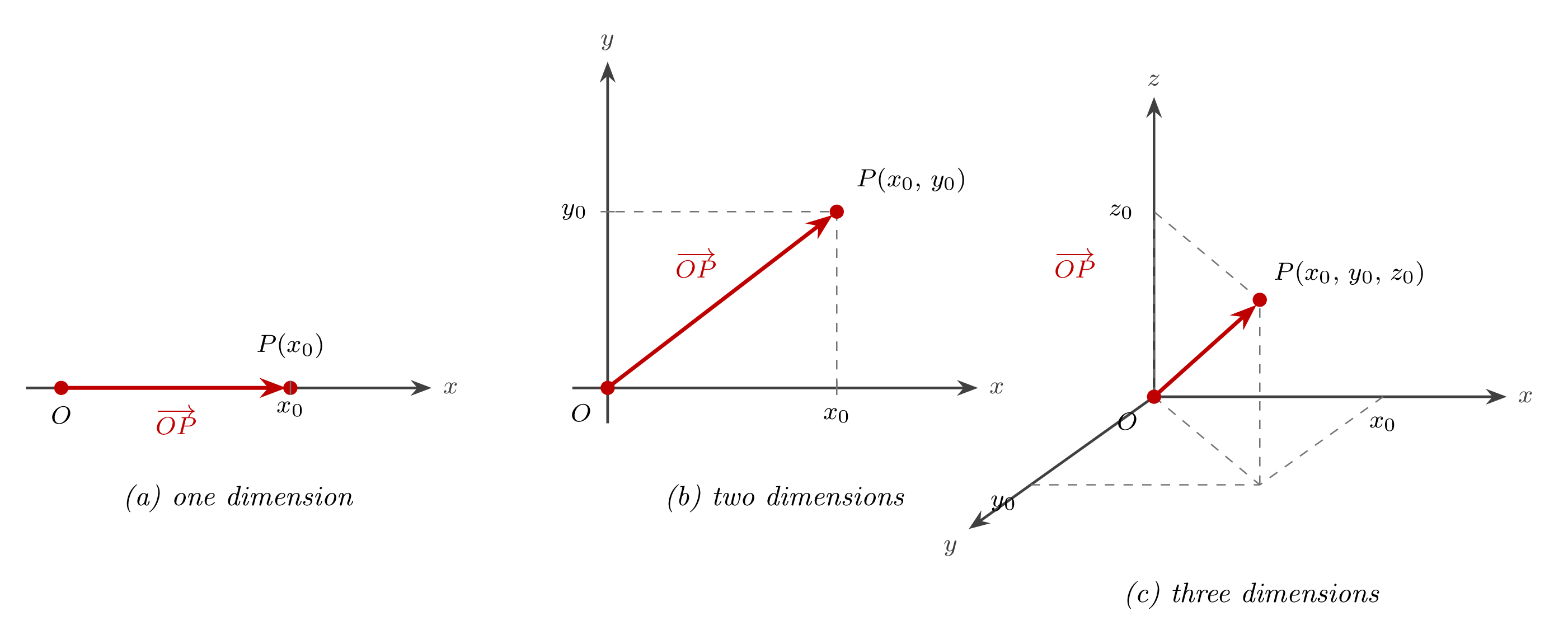
One-, two-, and three-dimensional coordinate systems showing a point P together with its position vector OP drawn as a directed arrow from the origin.

For $n = 1, 2, 3$ the geometric reading is the one the figure illustrates. A point $P$ in three-dimensional Euclidean space with Cartesian coordinates $(x_0, y_0, z_0)$ is associated with the $3 \times 1$ column

\begin{bmatrix} x_0 \\ y_0 \\ z_0 \end{bmatrix} \in \mathbb{R}^{3 \times 1},

and this column is exactly the position vector $\overrightarrow{OP}$ fixed to $P$ in Lesson 1PM and extended to $\mathbb{R}^3$ in Lesson 2AM. The arrow from the origin to $P$ and the column of its coordinates carry the same content; the two points of view will be used interchangeably. For $n \ge 4$ the arrow picture stops being available, but the column matrix still keeps the bookkeeping running, and that is the only reason the higher-dimensional arguments ahead remain tractable.

Length is imported without change. The magnitude $\|\mathbf{b}\|$ of a real column vector was defined from Pythagoras in Lesson 1AM and inherited by $\mathbb{R}^3$ in Lesson 2AM through the iterated-Pythagoras argument; the same Euclidean formula defines $\|\mathbf{b}\|$ for every $\mathbf{b} \in \mathbb{R}^{n \times 1}$ , no alteration required.

Problem 31

Take the system

\begin{cases} 2x_1 + x_2 - 3x_3 + x_4 = 5, \\ x_1 - x_2 + 4x_3 + 2x_4 = -1, \\ 3x_1 + 2x_2 + x_3 - x_4 = 0. \end{cases}

Write down its coefficient matrix $A$ and right-hand side column $\mathbf{b}$ , name the field $\mathbb{F}$ for which the system lives in $\mathbb{F}^{m \times n}$ and $\mathbb{F}^{m \times 1}$ , and decide which (if any) of the labels “square”, “upper triangular”, “lower triangular”, “diagonal”, “symmetric” apply to $A$ . Justify each rejection by producing an entry that violates the corresponding condition.

Addition and Scalar Multiplication

A vector of length $n$ is a matrix with one row or one column, and its addition and scalar multiplication were fixed entry by entry in Lesson 1AM and inherited by $\mathbb{R}^3$ without change in Lesson 2AM. Widening the rectangle from one row or column to $m \times n$ requires no new idea: we define addition and scaling on matrices the same way, entry by entry, and the previous geometric readings, parallelogram law and directed rescaling, survive untouched on the thin-matrix cases.

Definition 44 (Matrix Addition)

Let $A = [a_{ij}]$ and $B = [b_{ij}]$ both lie in $\mathbb{F}^{m \times n}$ . Their sum is the $m \times n$ matrix

A + B = [a_{ij} + b_{ij}]_{i,\, j = 1}^{m,\, n}.

The operation is defined only when $A$ and $B$ have the same size; mismatched sizes have no sum.

Restricted to column or row matrices the formula reproduces the componentwise vector addition of Lesson 1AM, together with the parallelogram-law reading illustrated there. Subtraction is introduced by the same device as in $\mathbb{F}$ : the difference $A - B$ is the unique $X \in \mathbb{F}^{m \times n}$ for which $X + B = A$ , namely $X = [a_{ij} - b_{ij}]$ . The $m \times n$ zero matrix $\mathbf{0}$ is the additive identity: $A + \mathbf{0} = A$ and $A - \mathbf{0} = A$ for every $A \in \mathbb{F}^{m \times n}$ .

Theorem 46 (Algebra of Matrix Addition)

For $A, B, C \in \mathbb{F}^{m \times n}$ ,

A + B = B + A, \qquad (A + B) + C = A + (B + C).

Proof

Every entry of $A + B$ is the scalar $a_{ij} + b_{ij}$ , and every entry of $B + A$ is $b_{ij} + a_{ij}$ ; these coincide because addition in $\mathbb{F}$ is commutative, one of the nine field axioms carried over from $\mathbb{R}$ to any $\mathbb{F}$ at the close of Lesson 3AM. The same argument applied to $(a_{ij} + b_{ij}) + c_{ij} = a_{ij} + (b_{ij} + c_{ij})$ handles associativity.

■

Shape is preserved under addition: the sum of two upper (respectively lower) triangular matrices of the same order is upper (respectively lower) triangular, and the sum of two diagonal matrices of the same order is diagonal, since the zero pattern on the relevant side of the main diagonal is carried through the entrywise sum unchanged.

Definition 45 (Scalar Multiplication of a Matrix)

For $A = [a_{ij}] \in \mathbb{F}^{m \times n}$ and $\alpha \in \mathbb{F}$ , the scalar multiple $\alpha A$ is the $m \times n$ matrix

\alpha A = [\alpha\, a_{ij}]_{i,\, j = 1}^{m,\, n}.

We write $-A$ for $(-1)A$ , so that $A - B = A + (-B)$ .

Restricted to columns or rows the formula reproduces the scalar multiplication of vectors from Lesson 1AM, and for real $\alpha$ the geometry illustrated there applies unchanged: the length of $\alpha\mathbf{a}$ is $|\alpha|$ times the length of $\mathbf{a}$ , with the direction preserved when $\alpha > 0$ and reversed when $\alpha < 0$ .

Theorem 47 (Algebra of Scalar Multiplication)

For $A, B \in \mathbb{F}^{m \times n}$ and $\alpha, \beta \in \mathbb{F}$ ,

0 A = \mathbf{0}, \qquad (\alpha + \beta) A = \alpha A + \beta A, \qquad \alpha(A + B) = \alpha A + \alpha B, \qquad \alpha(\beta A) = (\alpha\beta) A.

Proof

Each identity holds entrywise from a single field axiom applied to the scalars $\alpha, \beta, a_{ij}, b_{ij}$ : annihilation $0 \cdot a_{ij} = 0$ for the first, distributivity of $\mathbb{F}$ for the second and third, and associativity of multiplication in $\mathbb{F}$ for the fourth.

■

Example 50 (Adding and Scaling Matrices)

Let

A = \begin{bmatrix} 2 & -1 & 0 \\ 3 & 4 & 1 \end{bmatrix}, \qquad B = \begin{bmatrix} 1 & 2 & -3 \\ 0 & 1 & 5 \end{bmatrix}.

Then

A + B = \begin{bmatrix} 3 & 1 & -3 \\ 3 & 5 & 6 \end{bmatrix}, \qquad 2A - 3B = \begin{bmatrix} 1 & -8 & 9 \\ 6 & 5 & -13 \end{bmatrix},

while pairing $A$ with a $3 \times 2$ matrix would leave $A + \cdot$ undefined, the sizes not agreeing.

Matrix Multiplication

The $m \times n$ system packaged at the close of Lesson 3AM writes the $i$ th equation as

a_{i1} x_1 + a_{i2} x_2 + \cdots + a_{in} x_n = \sum_{k = 1}^{n} a_{ik} x_k = b_i,

a scalar entirely determined by the $i$ th row of the coefficient matrix $A$ and the column $\mathbf{x}$ of unknowns. Collecting all $m$ scalars into a single column recovers the right-hand side $\mathbf{b}$ . Any operation that packages $A$ and $\mathbf{x}$ into a product $A\mathbf{x}$ must reproduce exactly this “row into column” pairing, and the definition below is the unique extension of that rule to arbitrary conformable matrices.

Definition 46 (Matrix Product)

Let $A = [a_{ij}] \in \mathbb{F}^{m \times l}$ and $B = [b_{ij}] \in \mathbb{F}^{l \times n}$ ; here the column count of $A$ and the row count of $B$ agree, and $A, B$ are called conformable in this order. Their product is the $m \times n$ matrix $AB = [c_{ij}]$ with entries

c_{ij} = a_{i1} b_{1j} + a_{i2} b_{2j} + \cdots + a_{il} b_{lj} = \sum_{k = 1}^{l} a_{ik}\, b_{kj}, \qquad 1 \le i \le m, \quad 1 \le j \le n.

When the column count of $A$ does not match the row count of $B$ , the product $AB$ is not defined.

Remark (Row-Into-Column as a Special Case)

\mathbf{r} = \begin{bmatrix} a_1 & a_2 & \cdots & a_l \end{bmatrix} \in \mathbb{F}^{1 \times l}, \qquad \mathbf{c} = \begin{bmatrix} b_1 \\ b_2 \\ \vdots \\ b_l \end{bmatrix} \in \mathbb{F}^{l \times 1},

then $\mathbf{r}\mathbf{c}$ is a $1 \times 1$ matrix whose single entry is

a_1 b_1 + a_2 b_2 + \cdots + a_l b_l.

Over $\mathbb{R}$ this is exactly the familiar dot product of the corresponding vectors.

Computationally, $c_{ij}$ is obtained by pairing the $i$ th row of $A$ with the $j$ th column of $B$ and summing the products one index at a time. For the system of Lesson 3AM the product $A\mathbf{x}$ is precisely the column of left-hand sides of the equations, so the entire $m \times n$ system collapses to the single identity

A\mathbf{x} = \mathbf{b}.

This reformulation is the whole reason matrix multiplication is fixed the way it is. Every existence, uniqueness, and structure question from Lesson 3AM is now a question about a single equation in the matrix variable $\mathbf{x}$ .

Example 51 (A First Row-Into-Column Product)

Let

A = \begin{bmatrix} 2 & -1 & 0 \\ 0 & 3 & 1 \end{bmatrix}, \qquad B = \begin{bmatrix} 3 & 0 \\ 2 & 1 \\ 1 & 0 \end{bmatrix}.

The column count of $A$ and the row count of $B$ both equal $3$ , so $AB$ lies in $\mathbb{R}^{2 \times 2}$ . Pairing each row of $A$ with each column of $B$ ,

(AB)_{11} = 2(3) + (-1)(2) + 0(1) = 4, \quad (AB)_{12} = 2(0) + (-1)(1) + 0(0) = -1,

(AB)_{21} = 0(3) + 3(2) + 1(1) = 7, \quad (AB)_{22} = 0(0) + 3(1) + 1(0) = 3,

AB = \begin{bmatrix} 4 & -1 \\ 7 & 3 \end{bmatrix}.

The reverse product $BA$ is also conformable, since the column count of $B$ and the row count of $A$ both equal $2$ , but $BA$ lands in $\mathbb{R}^{3 \times 3}$ : the two products live in different spaces, and the question of whether $AB = BA$ is, here, meaningless.

Theorem 48 (The Identity Acts as a Unit)

Let $I_m, I_n$ denote the identity matrices of orders $m$ and $n$ . For every $A \in \mathbb{F}^{m \times n}$ ,

I_m A = A, \qquad A I_n = A.

In particular, $IA = AI = A$ whenever $A$ is square of the same order as $I$ .

Proof

The $(i,k)$ entry of $I_m$ is $1$ when $i = k$ and $0$ otherwise. Therefore

(I_m A)_{ij} = \sum_{k = 1}^{m} (I_m)_{ik}\, a_{kj} = a_{ij},

since only the term $k = i$ survives. The argument for $A I_n$ is identical: in

(A I_n)_{ij} = \sum_{k = 1}^{n} a_{ik}\, (I_n)_{kj},

only the term $k = j$ survives.

■

Theorem 49 (Distributive and Associative Laws)

For matrices of sizes such that every product and sum below is defined,

A(B + C) = AB + AC, \qquad (B + C) D = BD + CD, \qquad A(BC) = (AB)C.

Proof

Fix $A \in \mathbb{F}^{m \times l}$ and $B, C \in \mathbb{F}^{l \times n}$ . For the left distributive law,

\bigl(A(B + C)\bigr)_{ij} = \sum_{k = 1}^{l} a_{ik}(b_{kj} + c_{kj}) = \sum_{k = 1}^{l} a_{ik} b_{kj} + \sum_{k = 1}^{l} a_{ik} c_{kj} = (AB)_{ij} + (AC)_{ij},

using distributivity of multiplication over addition in $\mathbb{F}$ . The right distributive law is symmetric.

For associativity take $A \in \mathbb{F}^{m \times l}$ , $B \in \mathbb{F}^{l \times p}$ , $C \in \mathbb{F}^{p \times n}$ , so that all three products $AB$ , $BC$ , $(AB)C$ , $A(BC)$ are defined. Then

\bigl((AB)C\bigr)_{ij} = \sum_{r = 1}^{p} (AB)_{ir}\, c_{rj} = \sum_{r = 1}^{p} \Bigl(\sum_{k = 1}^{l} a_{ik} b_{kr}\Bigr) c_{rj} = \sum_{k = 1}^{l} a_{ik} \Bigl(\sum_{r = 1}^{p} b_{kr} c_{rj}\Bigr) = \bigl(A(BC)\bigr)_{ij},

the middle equality swapping the order of the two finite sums, legitimate in any field.

■

Matrix multiplication loses several properties that scalar multiplication enjoyed. The failures are cumulative, and the sharpest of them is the following.

Theorem 50 (Matrix Multiplication is Not Commutative)

For every $n \ge 2$ , there exist square matrices $A, B \in \mathbb{F}^{n \times n}$ with $AB \neq BA$ .

Proof

Take $n = 2$ and

A = \begin{bmatrix} 2 & 1 \\ 0 & 0 \end{bmatrix}, \qquad B = \begin{bmatrix} 1 & 0 \\ -1 & 0 \end{bmatrix}.

Direct computation gives

AB = \begin{bmatrix} 1 & 0 \\ 0 & 0 \end{bmatrix}, \qquad BA = \begin{bmatrix} 2 & 1 \\ -2 & -1 \end{bmatrix},

which disagree at every entry outside the $(1, 1)$ position. Padding $A$ and $B$ with zeros embeds the same witness into $\mathbb{F}^{n \times n}$ for every $n \ge 2$ .

■

Remark

Two further failures are worth recording. The product of two non-zero matrices may vanish: the choice

A = \begin{bmatrix} 1 & 0 \\ 0 & 0 \end{bmatrix}, \qquad B = \begin{bmatrix} 0 & 0 \\ 0 & 1 \end{bmatrix}

gives $AB = \mathbf{0}$ , so non-zero matrices can multiply to zero. Cancellation fails too: if $AB = AC$ with $A \neq \mathbf{0}$ , it need not follow that $B = C$ . With the same $A$ as above, any two matrices $B, C$ that agree on their first row but differ on their second satisfy $AB = AC$ , because the zero second row of $A$ annihilates every disagreement in the second row of $B$ and $C$ .

Having a well-behaved notion of product, and an identity $I$ that acts as a unit, permits iterating the operation.

Definition 47 (Powers of a Square Matrix)

Let $A \in \mathbb{F}^{n \times n}$ be square. For every positive integer $p$ set

A^p = \underbrace{A A \cdots A}_{p \text{ factors}},

and define $A^0 = I$ and $A^1 = A$ .

Theorem 51 (Exponent Laws for Matrix Powers)

For $A \in \mathbb{F}^{n \times n}$ and non-negative integers $p, q$ ,

A^p A^q = A^{p + q}, \qquad (A^p)^q = A^{pq}.

Remark (A Word on Induction)

A few arguments in this lesson depend on a positive integer parameter, such as an exponent $p$ . In such cases we will sometimes use mathematical induction, an important proof technique that we will study properly later in MCEA and again in MA1B.

For now, the version we need is simple:

first verify the statement at an initial value, usually $p = 0$ or $p = 1$ ;
then show that if the statement holds for one value $p = k$ , it must also hold for the next value $p = k + 1$ .

Once these two steps are established, the statement follows for every integer from the starting point onward. In the present lesson we use induction only in this basic step-by-step form.

Proof

Fix $p$ and induct on $q$ for the first identity. The base case $q = 0$ reads $A^p I = A^p$ , which is the identity acting as a unit. For the inductive step,

A^p A^{q + 1} = A^p (A^q A) = (A^p A^q) A = A^{p + q} A = A^{(p + q) + 1},

by associativity of matrix multiplication and the inductive hypothesis. Induct on $q$ for the second identity. The base case $q = 0$ reads $(A^p)^0 = I = A^0 = A^{p \cdot 0}$ . For the inductive step,

(A^p)^{q + 1} = (A^p)^q A^p = A^{pq} A^p = A^{pq + p} = A^{p(q + 1)},

by the inductive hypothesis and the first exponent law.

■

Example 52 (Cubing a Small Upper-Triangular Matrix)

Let $A = \begin{bmatrix} 2 & -1 \\ 0 & 2 \end{bmatrix}$ . Then

A^2 = \begin{bmatrix} 2 & -1 \\ 0 & 2 \end{bmatrix} \begin{bmatrix} 2 & -1 \\ 0 & 2 \end{bmatrix} = \begin{bmatrix} 4 & -4 \\ 0 & 4 \end{bmatrix}, \qquad A^3 = A \cdot A^2 = \begin{bmatrix} 8 & -12 \\ 0 & 8 \end{bmatrix}.

The upper-triangular shape of $A$ persists through every power. For $p \ge 1$ and indices $i > j$ , the entry $(A^p)_{ij}$ is a sum of products $a_{i k_1} a_{k_1 k_2} \cdots a_{k_{p-1} j}$ ; a non-zero such product would force $i \le k_1 \le k_2 \le \cdots \le k_{p-1} \le j$ , which contradicts $i > j$ .

Problem 32

Return to the system at the close of Lesson 3AM,

\begin{cases} x + y + z = 1, \\ x - y + 2z = 0, \end{cases}

and write it in the single-line form $A\mathbf{x} = \mathbf{b}$ by identifying the coefficient matrix $A$ and the right-hand side column $\mathbf{b}$ . Produce any particular column $\mathbf{x}_0 \in \mathbb{R}^{3 \times 1}$ that satisfies the system and verify by direct row-into-column multiplication that $A \mathbf{x}_0 = \mathbf{b}$ .

Problem 33

Let $\mathbf{a} \in \mathbb{F}^{m \times 1}$ be a column matrix and $\mathbf{c} \in \mathbb{F}^{1 \times n}$ a row matrix. Show that the product $\mathbf{a}\mathbf{c}$ , in this order, is defined and lies in $\mathbb{F}^{m \times n}$ , and write out the $(i, j)$ entry of $\mathbf{a}\mathbf{c}$ in terms of the components of $\mathbf{a}$ and $\mathbf{c}$ . This matrix is called an outer product of $\mathbf{a}$ and $\mathbf{c}$ .

Problem 34

Let $A \in \mathbb{F}^{m \times l}$ have columns $\mathbf{a}_1, \mathbf{a}_2, \ldots, \mathbf{a}_l \in \mathbb{F}^{m \times 1}$ , and let $B \in \mathbb{F}^{l \times n}$ have rows $\mathbf{r}_1, \mathbf{r}_2, \ldots, \mathbf{r}_l \in \mathbb{F}^{1 \times n}$ . Using the outer-product construction of the previous problem, prove the column-row decomposition

AB = \sum_{k = 1}^{l} \mathbf{a}_k \mathbf{r}_k,

where each summand $\mathbf{a}_k \mathbf{r}_k$ is an $m \times n$ outer product. Compare this expression with the row-into-column formula that defines $AB$ directly, and convince yourself that the two points of view compute the same entries.

The failure of commutativity in the earlier noncommutativity theorem is the source of most of the subtlety in matrix algebra, so it pays to name the cases where commutation is restored and the shapes whose self-multiplication behaves in an unusually rigid way. Four labels below cover the patterns that will reappear throughout the rest of the course.

Commuting Matrices

Definition 48 (Commuting Matrices)

Square matrices $A, B \in \mathbb{F}^{n \times n}$ commute when $AB = BA$ . The difference $[A, B] = AB - BA$ is the commutator of $A$ and $B$ , and $A$ and $B$ commute exactly when $[A, B] = 0$ .

Commutation is the exception, not the rule; the earlier noncommutativity theorem already supplied a $2 \times 2$ counterexample, and every computation with two generic matrices should start from the assumption that order matters. The results below are the standard reasons commutation is recovered in practice.

Theorem 52

For any $A \in \mathbb{F}^{n \times n}$ and any scalar $\lambda \in \mathbb{F}$ , the matrix $\lambda I_n$ commutes with $A$ :

A(\lambda I_n) = \lambda A = (\lambda I_n) A.

Proof

The $(i, j)$ entry of $A(\lambda I_n)$ is

\sum_{k=1}^n a_{ik}(\lambda I_n)_{kj},

and all terms vanish except the one with $k=j$ , because the only non-zero entry in column $j$ of $\lambda I_n$ is the diagonal entry $\lambda$ . Hence $(A(\lambda I_n))_{ij} = \lambda a_{ij}$ . Likewise,

((\lambda I_n)A)_{ij} = \sum_{k=1}^n (\lambda I_n)_{ik} a_{kj},

and all terms vanish except the one with $k=i$ , so $((\lambda I_n)A)_{ij} = \lambda a_{ij}$ . Both therefore agree with the $(i,j)$ entry of $\lambda A$ .

■

Problem 35

Show that a matrix $S \in \mathbb{F}^{n \times n}$ commutes with every square matrix in $\mathbb{F}^{n \times n}$ if and only if $S$ is a scalar matrix $aI_n$ for some $a \in \mathbb{F}$ .

Theorem 53 (Diagonal Matrices Commute)

D = \operatorname{diag}(d_1, d_2, \ldots, d_n), \qquad E = \operatorname{diag}(e_1, e_2, \ldots, e_n),

then

DE = ED = \operatorname{diag}(d_1 e_1, d_2 e_2, \ldots, d_n e_n).

Proof

Since every off-diagonal entry of $D$ and $E$ is zero, the product of row $i$ with column $j$ vanishes when $i \neq j$ , so both $DE$ and $ED$ are diagonal. On the diagonal,

(DE)_{ii} = d_i e_i = e_i d_i = (ED)_{ii},

because multiplication in $\mathbb{F}$ is commutative.

■

Theorem 54 (Commuting with a Diagonal Matrix of Distinct Entries)

Let

D = \operatorname{diag}(d_1, d_2, \ldots, d_n) \in \mathbb{F}^{n \times n}

with $d_i \neq d_j$ whenever $i \neq j$ . If $A = [a_{ij}] \in \mathbb{F}^{n \times n}$ satisfies $AD = DA$ , then $A$ is diagonal.

Proof

The $(i,j)$ entry of $AD$ is $a_{ij} d_j$ , while the $(i,j)$ entry of $DA$ is $d_i a_{ij}$ . Hence

a_{ij} d_j = d_i a_{ij},

(d_j - d_i)a_{ij} = 0.

If $i \neq j$ , then $d_j - d_i \neq 0$ , and since we are working in a field this forces $a_{ij} = 0$ . Thus every off-diagonal entry of $A$ is zero, so $A$ is diagonal.

■

Theorem 55

If $A, B \in \mathbb{F}^{n \times n}$ commute, then $A^p B = B A^p$ for every $p \ge 0$ , and more generally $A^p B^q = B^q A^p$ for every $p, q \ge 0$ .

Proof

Fix $B$ and induct on $p$ . The base $p = 0$ reads $IB = B = BI$ . For the step,

A^{p+1} B = A(A^p B) = A(B A^p) = (AB) A^p = (BA) A^p = B A^{p+1},

using the inductive hypothesis at the second equality and commutation at the fourth. A symmetric induction on $q$ gives $A B^q = B^q A$ , and combining the two yields $A^p B^q = B^q A^p$ .

■

Theorem 56 (The Commutant Is Closed)

Fix $A \in \mathbb{F}^{n \times n}$ and let $C(A) = \{X \in \mathbb{F}^{n \times n} : AX = XA\}$ be its commutant. If $X, Y \in C(A)$ and $\alpha \in \mathbb{F}$ , then $X + Y$ , $\alpha X$ , and $XY$ all lie in $C(A)$ .

Proof

From $AX = XA$ and $AY = YA$ : $A(X + Y) = AX + AY = XA + YA = (X + Y)A$ ; $A(\alpha X) = \alpha AX = \alpha XA = (\alpha X) A$ ; and $A(XY) = (AX)Y = (XA)Y = X(AY) = X(YA) = (XY) A$ . The first two computations use distributivity and scalar compatibility, and the last uses associativity of matrix multiplication together with the commutation hypotheses.

■

Example 53 (Commutant of a Diagonal Matrix)

Find every $B \in \mathbb{R}^{2 \times 2}$ that commutes with

A = \begin{bmatrix} 2 & 0 \\ 0 & 3 \end{bmatrix}.

Write $B = \begin{bmatrix} p & q \\ r & s \end{bmatrix}$ . Then

AB = \begin{bmatrix} 2p & 2q \\ 3r & 3s \end{bmatrix}, \qquad BA = \begin{bmatrix} 2p & 3q \\ 2r & 3s \end{bmatrix},

so $AB = BA$ forces $2q = 3q$ and $3r = 2r$ , that is $q = r = 0$ , while $p, s$ remain free. The commutant is

C(A) = \left\{ \begin{bmatrix} p & 0 \\ 0 & s \end{bmatrix} : p, s \in \mathbb{R} \right\}.

Were the two diagonal entries of $A$ equal, the calculation would instead return every $2 \times 2$ matrix, in agreement with the scalar-matrix commuting theorem above.

Problem 36

Determine every $B \in \mathbb{R}^{2 \times 2}$ that commutes with

A = \begin{bmatrix} 1 & 1 \\ 0 & 1 \end{bmatrix},

and describe what changes, compared with the diagonal example just above, once the off-diagonal entry is introduced.

Idempotent Matrices

A matrix whose square returns itself is the algebraic shape every projection in the course will turn out to have.

Definition 49 (Idempotent Matrix)

A square matrix $A \in \mathbb{F}^{n \times n}$ is idempotent when $A^2 = A$ . Both $I_n$ and $\mathbf{0}_n$ are idempotent by inspection, and induction on $p$ gives $A^p = A$ for every $p \ge 1$ .

Example 54 (A Non-Trivial Idempotent)

The matrix

A = \begin{bmatrix} 1 & 2 & 2 \\ 0 & 0 & -1 \\ 0 & 0 & 1 \end{bmatrix}

satisfies $A^2 = A$ . The rows of $A^2$ are read off row-into-column: row one of $A$ times the columns of $A$ gives $(1, 2, 1 \cdot 2 + 2 \cdot (-1) + 2 \cdot 1) = (1, 2, 2)$ , row two gives $(0, 0, 0 \cdot 2 + 0 \cdot (-1) + (-1) \cdot 1) = (0, 0, -1)$ , and row three gives $(0, 0, 0 \cdot 2 + 0 \cdot (-1) + 1 \cdot 1) = (0, 0, 1)$ . Stacking these reproduces $A$ . The matrix is neither $\mathbf{0}$ nor $I$ , so idempotence is genuinely richer than the two trivial endpoints.

Theorem 57 (The Complementary Idempotent)

If $A \in \mathbb{F}^{n \times n}$ is idempotent, so is $I_n - A$ , and the two matrices annihilate each other:

A(I_n - A) = (I_n - A) A = \mathbf{0}.

Proof

Using the unit and distributive laws established earlier,

(I - A)^2 = I - 2A + A^2 = I - 2A + A = I - A,

so $I - A$ is idempotent. For the orthogonality, $A(I - A) = A - A^2 = A - A = \mathbf{0}$ , and $(I - A)A = A - A^2 = \mathbf{0}$ by the same cancellation.

■

Example 55 (A Projection and Its Complement)

Let

P = \begin{bmatrix} 1 & 0 \\ 0 & 0 \end{bmatrix}.

Then $P^2 = P$ , so $P$ is idempotent. Its complementary idempotent is

I_2 - P = \begin{bmatrix} 0 & 0 \\ 0 & 1 \end{bmatrix},

and indeed

P(I_2-P) = (I_2-P)P = \mathbf{0}.

These two matrices project onto the coordinate axes separately: left multiplication by $P$ keeps the first coordinate and kills the second, while left multiplication by $I_2-P$ does the opposite.

Problem 37

Let $A, B \in \mathbb{F}^{n \times n}$ be idempotent and commute. Prove that $AB$ is idempotent, and exhibit two idempotents in $\mathbb{R}^{2 \times 2}$ that do not commute and whose product is not idempotent, showing that the hypothesis $AB = BA$ is load-bearing rather than cosmetic.

Problem 38

Classify all idempotent matrices in $\mathbb{F}^{2 \times 2}$ . In other words, determine all

A = \begin{bmatrix} a & b \\ c & d \end{bmatrix}

for which $A^2 = A$ .

Nilpotent Matrices

Opposite to idempotents, for which repeated multiplication stabilises, are matrices whose repeated multiplication annihilates them outright.

Definition 50 (Nilpotent Matrix)

A square matrix $A \in \mathbb{F}^{n \times n}$ is nilpotent when there is an integer $p \ge 1$ with $A^p = \mathbf{0}$ . The smallest such $p$ is the index of nilpotence of $A$ .

Example 56 (Strictly Upper-Triangular Nilpotent)

The matrix

N = \begin{bmatrix} 0 & 1 & 0 \\ 0 & 0 & 1 \\ 0 & 0 & 0 \end{bmatrix}

satisfies

N^2 = \begin{bmatrix} 0 & 0 & 1 \\ 0 & 0 & 0 \\ 0 & 0 & 0 \end{bmatrix}, \qquad N^3 = \mathbf{0}_3,

so $N$ is nilpotent with index $3$ . Each successive power pushes the non-zero band one step further above the main diagonal until it exits the matrix.

Theorem 58 (Strictly Triangular Matrices Are Nilpotent)

Every strictly upper-triangular $A \in \mathbb{F}^{n \times n}$ , meaning $a_{ij} = 0$ whenever $i \ge j$ , satisfies $A^n = \mathbf{0}$ .

Proof

We prove by induction on $p \ge 1$ that

(A^p)_{ij} = 0 \qquad \text{whenever } j-i < p.

For $p=1$ this is exactly the assumption that $A$ is strictly upper-triangular: if $j-i<1$ , then $j \le i$ , so $a_{ij}=0$ .

Now assume the claim for some $p$ . Then

(A^{p+1})_{ij} = \sum_{k=1}^n (A^p)_{ik} a_{kj}.

For a term $(A^p)_{ik} a_{kj}$ to be non-zero, the induction hypothesis forces $k-i \ge p$ , and strict upper-triangularity forces $j-k \ge 1$ . Adding gives

j-i = (j-k) + (k-i) \ge 1 + p = p+1.

So if $j-i < p+1$ , every term in the sum is zero, and hence $(A^{p+1})_{ij}=0$ . This proves the induction step.

Finally, in an $n \times n$ matrix we always have $j-i \le n-1$ . Therefore when $p=n$ the inequality $j-i < n$ holds for every pair $(i,j)$ , so every entry of $A^n$ is zero. Hence $A^n = \mathbf{0}$ .

The same argument, with the inequalities reversed, handles the strictly lower-triangular case.

■

Problem 39

Show that if $A \in \mathbb{F}^{n \times n}$ is nilpotent with $A^p = \mathbf{0}$ , then

(I_n - A)(I_n + A + A^2 + \cdots + A^{p - 1}) = I_n.

Deduce that a nilpotent matrix can never equal $I_n$ , and exhibit a non-zero $B \in \mathbb{R}^{2 \times 2}$ with $B^2 = \mathbf{0}$ to confirm that the nilpotent class is non-empty beyond the zero matrix.

Problem 40

Classify all nilpotent matrices in $\mathbb{F}^{2 \times 2}$ . Determine separately which ones have index of nilpotence $1$ and which have index of nilpotence $2$ .

Involutory Matrices

Definition 51 (Involutory Matrix)

A square matrix $A \in \mathbb{F}^{n \times n}$ is involutory when $A^2 = I_n$ . Geometrically, multiplication by $A$ is its own undoing; algebraically, $A$ will turn out to be its own inverse once the inverse is defined in a later lesson.

Example 57 (The Swap Matrix Is Involutory)

The matrix

J = \begin{bmatrix} 0 & 1 \\ 1 & 0 \end{bmatrix}

has

J^2 = \begin{bmatrix} 0 \cdot 0 + 1 \cdot 1 & 0 \cdot 1 + 1 \cdot 0 \\ 1 \cdot 0 + 0 \cdot 1 & 1 \cdot 1 + 0 \cdot 0 \end{bmatrix} = \begin{bmatrix} 1 & 0 \\ 0 & 1 \end{bmatrix} = I_2,

so $J$ is involutory. Acting on a column by left multiplication, $J$ swaps the two entries, and performing the swap twice returns the original column.

Theorem 59 (Powers of an Involutory Matrix)

If $A \in \mathbb{F}^{n \times n}$ is involutory, then $A^{2k} = I_n$ and $A^{2k + 1} = A$ for every $k \ge 0$ .

Proof

Induct on $k$ , with $A^0 = I$ and $A^1 = A$ as bases. For the even step, $A^{2(k+1)} = A^{2k} A^2 = I \cdot I = I$ , and for the odd step, $A^{2(k+1)+1} = A^{2k+1} A^2 = A \cdot I = A$ , using $A^2 = I$ at each closure.

■

Theorem 60 (Idempotent Splitting of an Involution)

Let $A \in \mathbb{F}^{n \times n}$ be involutory and suppose $\tfrac{1}{2} \in \mathbb{F}$ , which holds for $\mathbb{F} = \mathbb{R}$ and $\mathbb{F} = \mathbb{C}$ . The matrices

P_+ = \tfrac{1}{2}(I_n + A), \qquad P_- = \tfrac{1}{2}(I_n - A)

are idempotent and satisfy $P_+ + P_- = I_n$ , $P_+ - P_- = A$ , and $P_+ P_- = P_- P_+ = \mathbf{0}$ .

Proof

Using $A^2 = I$ ,

P_+^2 = \tfrac{1}{4}(I + A)^2 = \tfrac{1}{4}(I + 2A + A^2) = \tfrac{1}{4}(2I + 2A) = \tfrac{1}{2}(I + A) = P_+,

and the symmetric calculation gives $P_-^2 = P_-$ . The sum and difference are by direct expansion, and

P_+ P_- = \tfrac{1}{4}(I + A)(I - A) = \tfrac{1}{4}(I - A^2) = \mathbf{0},

with $P_- P_+ = \mathbf{0}$ by the same cancellation.

■

Example 58 (A Reflection Splits into Two Projections)

Take

A = \begin{bmatrix} 1 & 0 \\ 0 & -1 \end{bmatrix}.

Then $A^2 = I_2$ , so $A$ is involutory. The associated idempotents are

P_+ = \tfrac{1}{2}(I_2 + A) = \begin{bmatrix} 1 & 0 \\ 0 & 0 \end{bmatrix}, \qquad P_- = \tfrac{1}{2}(I_2 - A) = \begin{bmatrix} 0 & 0 \\ 0 & 1 \end{bmatrix}.

So this involution is exactly the difference of two complementary coordinate projections:

A = P_+ - P_-.

Geometrically, $A$ fixes the $x$ -axis and flips the sign on the $y$ -axis.

Remark

An involution can also be characterized by the factorization

A^2 = I_n \qquad\Longleftrightarrow\qquad (I_n - A)(I_n + A) = \mathbf{0}.

Indeed,

(I_n - A)(I_n + A) = I_n + A - A - A^2 = I_n - A^2,

since $I_n$ commutes with $A$ . So either condition is exactly the statement $I_n - A^2 = \mathbf{0}$ .

Problem 41

Verify that

A = \begin{bmatrix} 4 & 3 \\ -5 & -4 \end{bmatrix}

is involutory, and write down the idempotents $P_\pm = \tfrac{1}{2}(I_2 \pm A)$ from the idempotent-splitting theorem above for this $A$ .

Problem 42

For any real angle $\theta$ , show that

A = \begin{bmatrix} \cos \theta & \sin \theta \\ \sin \theta & -\cos \theta \end{bmatrix}

is involutory. Reminder:

\cos^2 \theta + \sin^2 \theta = 1.

Problem 43

Let $J_n$ be the $n \times n$ matrix with $1$ in every position on the secondary diagonal and $0$ elsewhere. Show that $J_n$ is involutory, and conclude that $-J_n$ is also involutory.

Problem 44

Prove that if $A, B \in \mathbb{F}^{n \times n}$ are involutory and commute, then $AB$ is involutory. Exhibit a $2 \times 2$ example showing that the conclusion fails once commutation is dropped.

Problem 45

Assume $\tfrac{1}{2} \in \mathbb{F}$ , for example $\mathbb{F} = \mathbb{R}$ or $\mathbb{C}$ . Classify all involutory matrices in $\mathbb{F}^{2 \times 2}$ . That is, determine all

A = \begin{bmatrix} a & b \\ c & d \end{bmatrix}

for which $A^2 = I_2$ .

Transpose and Conjugate Transpose

The previous section left one asymmetry untouched: a column of length $n$ and a row carrying the same entries are genuinely distinct objects in $\mathbb{F}^{n \times 1}$ and $\mathbb{F}^{1 \times n}$ because their sizes differ. The transpose is the explicit bridge between the two, and upgraded to complex matrices it becomes the conjugate transpose, the operation that the Hermitian and symmetric conditions introduced earlier in this lesson were secretly measuring.

Definition 52 (Transpose)

The transpose of $A = [a_{ij}] \in \mathbb{F}^{m \times n}$ is the $n \times m$ matrix

A^{\top} = [a_{ji}]_{i,\, j = 1}^{n,\, m}

obtained by swapping rows and columns: the $(i, j)$ entry of $A^{\top}$ is the $(j, i)$ entry of $A$ . Thus, if

A = \begin{bmatrix} a_{11} & a_{12} & \cdots & a_{1n} \\ a_{21} & a_{22} & \cdots & a_{2n} \\ \vdots & \vdots & & \vdots \\ a_{m1} & a_{m2} & \cdots & a_{mn} \end{bmatrix},

then

A^{\top} = \begin{bmatrix} a_{11} & a_{21} & \cdots & a_{m1} \\ a_{12} & a_{22} & \cdots & a_{m2} \\ \vdots & \vdots & & \vdots \\ a_{1n} & a_{2n} & \cdots & a_{mn} \end{bmatrix}.

Two readings of the transpose are worth keeping side by side. The rows of $A^{\top}$ , read left to right, are the columns of $A$ , read top to bottom; and the columns of $A^{\top}$ are the rows of $A$ . Geometrically the operation is a reflection of the rectangle across its main diagonal.

The symmetric condition introduced earlier asks $a_{ji} = a_{ij}$ for every $i, j$ , which is precisely $A^{\top} = A$ , so a matrix is symmetric if and only if it equals its own transpose. The Hermitian condition $a_{ji} = \overline{a_{ij}}$ mixes transposition with conjugation, and it is restated cleanly only after the conjugate transpose is defined below.

Example 59 (Transposes of Small Matrices)

For

A = \begin{bmatrix} 1 & 2 & 3 \\ 4 & 5 & 6 \end{bmatrix}, \qquad \mathbf{b} = \begin{bmatrix} 1 \\ -2 \\ 3 \end{bmatrix},

direct reading gives

A^{\top} = \begin{bmatrix} 1 & 4 \\ 2 & 5 \\ 3 & 6 \end{bmatrix} \in \mathbb{R}^{3 \times 2}, \qquad \mathbf{b}^{\top} = \begin{bmatrix} 1 & -2 & 3 \end{bmatrix} \in \mathbb{R}^{1 \times 3}.

The transpose of a column is the row carrying the same entries, fulfilling the bridge promised in the earlier discussion of rows and columns.

Theorem 61 (Transpose Is an Involution)

For every $A \in \mathbb{F}^{m \times n}$ ,

(A^{\top})^{\top} = A.

Proof

The $(i, j)$ entry of $A^{\top}$ is $a_{ji}$ , so the $(i, j)$ entry of $(A^{\top})^{\top}$ is $a_{ij}$ , which is the $(i, j)$ entry of $A$ .

■

Theorem 62 (Transpose of Sum and Scalar Multiple)

For $A, B \in \mathbb{F}^{m \times n}$ and $\alpha \in \mathbb{F}$ ,

(A + B)^{\top} = A^{\top} + B^{\top}, \qquad (\alpha A)^{\top} = \alpha A^{\top}.

Proof

The $(i, j)$ entry of $(A + B)^{\top}$ is $(A + B)_{ji} = a_{ji} + b_{ji}$ , which is the $(i, j)$ entry of $A^{\top} + B^{\top}$ . The $(i, j)$ entry of $(\alpha A)^{\top}$ is $(\alpha A)_{ji} = \alpha a_{ji}$ , which is the $(i, j)$ entry of $\alpha A^{\top}$ .

■

Problem 46

If $A, B \in \mathbb{F}^{n \times n}$ are symmetric, show that $A + B$ is symmetric.

Theorem 63 (Transpose Reverses Products)

For $A \in \mathbb{F}^{m \times l}$ and $B \in \mathbb{F}^{l \times n}$ ,

(AB)^{\top} = B^{\top} A^{\top}.

More generally, for matrices $A_1, A_2, \ldots, A_k$ whose sizes make the product $A_1 A_2 \cdots A_k$ defined,

(A_1 A_2 \cdots A_k)^{\top} = A_k^{\top} \cdots A_2^{\top} A_1^{\top}.

Proof

The $(i, j)$ entry of $(AB)^{\top}$ is $(AB)_{ji} = \sum_{k = 1}^{l} a_{j k} b_{k i}$ , while the $(i, j)$ entry of $B^{\top} A^{\top}$ is

\sum_{k = 1}^{l} (B^{\top})_{ik} (A^{\top})_{kj} = \sum_{k = 1}^{l} b_{k i} a_{j k},

and the two sums agree termwise by commutativity of multiplication in $\mathbb{F}$ . The $k$ -fold identity follows by induction on $k$ , using the two-fold version together with the associativity of matrix multiplication established earlier.

■

Example 60 (Transposing a Product)

Let

A = \begin{bmatrix} 1 & 2 & 0 \\ -1 & 3 & 4 \end{bmatrix}, \qquad B = \begin{bmatrix} 2 & 1 \\ 0 & -1 \\ 5 & 2 \end{bmatrix}.

Then

AB = \begin{bmatrix} 2 & -1 \\ 18 & 4 \end{bmatrix}, \qquad\text{so}\qquad (AB)^{\top} = \begin{bmatrix} 2 & 18 \\ -1 & 4 \end{bmatrix}.

On the other hand,

B^{\top} = \begin{bmatrix} 2 & 0 & 5 \\ 1 & -1 & 2 \end{bmatrix}, \qquad A^{\top} = \begin{bmatrix} 1 & -1 \\ 2 & 3 \\ 0 & 4 \end{bmatrix},

and direct multiplication gives

B^{\top}A^{\top} = \begin{bmatrix} 2 & 18 \\ -1 & 4 \end{bmatrix} = (AB)^{\top}.

The order reversal is visible in the calculation: the transpose does not preserve the order of the factors.

Skew-Symmetric Matrices

Definition 53 (Skew-Symmetric Matrix)

A square matrix $A \in \mathbb{F}^{n \times n}$ is skew-symmetric when $A^{\top} = -A$ , equivalently $a_{ji} = -a_{ij}$ for every $1 \le i, j \le n$ . Setting $i = j$ gives $2 a_{ii} = 0$ , so whenever $\tfrac{1}{2} \in \mathbb{F}$ every diagonal entry of a skew-symmetric matrix is zero.

Example 61 (A Skew-Symmetric Matrix)

The matrix

S = \begin{bmatrix} 0 & 2 & -3 \\ -2 & 0 & 5 \\ 3 & -5 & 0 \end{bmatrix} \in \mathbb{R}^{3 \times 3}

is skew-symmetric: its diagonal is zero, and reflecting each off-diagonal entry across the main diagonal negates it.

Problem 47

Let $A \in \mathbb{F}^{n \times n}$ . Show that the matrices

AA^{\top}, \qquad A^{\top}A, \qquad A^{\top} + A

are symmetric, and that

A - A^{\top}

is skew-symmetric.

Theorem 64 (Symmetric-Skew Decomposition)

Assume $\tfrac{1}{2} \in \mathbb{F}$ . Every $A \in \mathbb{F}^{n \times n}$ admits a unique decomposition

A = S + K, \qquad S^{\top} = S, \quad K^{\top} = -K,

with $S$ symmetric and $K$ skew-symmetric, given by

S = \tfrac{1}{2}(A + A^{\top}), \qquad K = \tfrac{1}{2}(A - A^{\top}).

Proof

Existence. Using the transpose involution and the transpose sum rule,

S^{\top} = \tfrac{1}{2}(A^{\top} + A) = S, \qquad K^{\top} = \tfrac{1}{2}(A^{\top} - A) = -K,

and $S + K = \tfrac{1}{2}(A + A^{\top}) + \tfrac{1}{2}(A - A^{\top}) = A$ .

Uniqueness. Suppose $A = S' + K'$ with $S'$ symmetric and $K'$ skew-symmetric. Transposing gives $A^{\top} = S' - K'$ , and solving the two equations for $S'$ and $K'$ returns the formulas above, forcing $(S', K') = (S, K)$ .

■

Problem 48

For

A = \begin{bmatrix} 1 & 3 & -2 \\ 0 & 4 & 5 \\ 7 & -1 & 2 \end{bmatrix},

compute the symmetric matrix

S = \tfrac{1}{2}(A + A^{\top})

and the skew-symmetric matrix

K = \tfrac{1}{2}(A - A^{\top}),

and verify directly that $A = S + K$ .

Complex Conjugate and Conjugate Transpose

Over $\mathbb{C}$ the transpose by itself is not quite the right operation: the Hermitian condition introduced earlier mixes transposition with complex conjugation, and the pair needs both halves introduced explicitly before it can be used cleanly.

Definition 54 (Conjugate of a Matrix)

For $A = [a_{ij}] \in \mathbb{C}^{m \times n}$ the conjugate $\overline{A}$ is the $m \times n$ matrix whose $(i, j)$ entry is $\overline{a_{ij}}$ . Conjugation is the identity on $\mathbb{R}^{m \times n}$ , since real scalars are fixed by conjugation in $\mathbb{C}$ .

Definition 55 (Conjugate Transpose)

For $A \in \mathbb{C}^{m \times n}$ the conjugate transpose, written $A^{*}$ (also $A^{H}$ in some texts), is the $n \times m$ matrix

A^{*} = \overline{A^{\top}} = (\overline{A})^{\top},

that is, $(A^{*})_{ij} = \overline{a_{ji}}$ . Explicitly,

A^{*} = \begin{bmatrix} \overline{a_{11}} & \overline{a_{21}} & \cdots & \overline{a_{m1}} \\ \overline{a_{12}} & \overline{a_{22}} & \cdots & \overline{a_{m2}} \\ \vdots & \vdots & & \vdots \\ \overline{a_{1n}} & \overline{a_{2n}} & \cdots & \overline{a_{mn}} \end{bmatrix}.

Over $\mathbb{R}$ conjugation is trivial, so $A^{*}$ collapses to $A^{\top}$ .

The Hermitian condition introduced earlier now reads $A^{*} = A$ : a matrix is Hermitian precisely when it equals its own conjugate transpose, and over $\mathbb{R}$ this reduces further to $A^{\top} = A$ , the symmetric condition of the previous subsection.

Remark

The $1 \times 1$ complex matrices are just the complex numbers in matrix clothing:

\begin{bmatrix} z \end{bmatrix} \longleftrightarrow z \in \mathbb{C}.

Under this identification, the Hermitian condition becomes

\begin{bmatrix} z \end{bmatrix}^{*} = \begin{bmatrix} z \end{bmatrix} \qquad\Longleftrightarrow\qquad \overline{z} = z,

so the $1 \times 1$ Hermitian matrices are exactly the real numbers.

Example 62 (Conjugate Transpose of a Complex Matrix)

For

A = \begin{bmatrix} 1 + i & 2 \\ -3 i & 4 - i \end{bmatrix} \in \mathbb{C}^{2 \times 2},

transposing then conjugating gives

A^{\top} = \begin{bmatrix} 1 + i & -3 i \\ 2 & 4 - i \end{bmatrix}, \qquad A^{*} = \begin{bmatrix} 1 - i & 3 i \\ 2 & 4 + i \end{bmatrix}.

Conjugating first and then transposing produces the same result, illustrating the commutativity of the two operations built into the definition of conjugate transpose.

Theorem 65 (Conjugate Transpose Is an Involution)

For every $A \in \mathbb{C}^{m \times n}$ ,

(A^{*})^{*} = A.

Proof

The $(i, j)$ entry of $A^{*}$ is $\overline{a_{ji}}$ , so the $(i, j)$ entry of $(A^{*})^{*}$ is $\overline{\overline{a_{ij}}} = a_{ij}$ , using that conjugation in $\mathbb{C}$ is involutive.

■

Theorem 66 (Conjugate Transpose of Sum and Scalar Multiple)

For $A, B \in \mathbb{C}^{m \times n}$ and $\alpha \in \mathbb{C}$ ,

(A + B)^{*} = A^{*} + B^{*}, \qquad (\alpha A)^{*} = \overline{\alpha}\, A^{*}.

Proof

Entrywise, $((A + B)^{*})_{ij} = \overline{a_{ji} + b_{ji}} = \overline{a_{ji}} + \overline{b_{ji}}$ , matching $A^{*} + B^{*}$ . For the scalar, $((\alpha A)^{*})_{ij} = \overline{\alpha a_{ji}} = \overline{\alpha}\, \overline{a_{ji}}$ , matching $\overline{\alpha} A^{*}$ . The appearance of $\overline{\alpha}$ in place of $\alpha$ is the genuinely new feature once conjugation joins the transpose.

■

Theorem 67 (Conjugate Transpose Reverses Products)

For $A \in \mathbb{C}^{m \times l}$ and $B \in \mathbb{C}^{l \times n}$ ,

(AB)^{*} = B^{*} A^{*},

and more generally $(A_1 A_2 \cdots A_k)^{*} = A_k^{*} \cdots A_2^{*} A_1^{*}$ whenever the product is defined.

Proof

Combine the transpose-of-products theorem with entrywise conjugation:

(AB)^{*} = \overline{(AB)^{\top}} = \overline{B^{\top} A^{\top}} = \overline{B^{\top}}\, \overline{A^{\top}} = B^{*} A^{*},

where the third equality is checked entrywise:

\bigl(\overline{B^{\top} A^{\top}}\bigr)_{ij} = \overline{\sum_{k=1}^{l} (B^{\top})_{ik} (A^{\top})_{kj}} = \sum_{k=1}^{l} \overline{(B^{\top})_{ik}}\, \overline{(A^{\top})_{kj}} = \bigl(\overline{B^{\top}}\, \overline{A^{\top}}\bigr)_{ij}.

Thus conjugation commutes with transposition and respects matrix products because it respects sums and products of scalars in $\mathbb{C}$ . The $k$ -fold identity is by induction on $k$ .

■

Theorem 68 (Hermitian Combinations from a Complex Matrix)

For every $A \in \mathbb{C}^{n \times n}$ , the four matrices

A + A^{*}, \qquad i(A - A^{*}), \qquad A A^{*}, \qquad A^{*} A

are all Hermitian.

Proof

Use the involution rule for $^{*}$ together with the sum, scalar, and product rules above. First, $(A + A^{*})^{*} = A^{*} + (A^{*})^{*} = A^{*} + A$ . Second, $(i(A - A^{*}))^{*} = \overline{i}(A - A^{*})^{*} = -i(A^{*} - A) = i(A - A^{*})$ . For the last two, $(A A^{*})^{*} = (A^{*})^{*} A^{*} = A A^{*}$ , and the same argument with the roles of $A$ and $A^{*}$ swapped handles $A^{*} A$ .

■

Example 63 (Hermitian Combinations in Practice)

Let

A = \begin{bmatrix} 1+i & 2 \\ -3i & 4-i \end{bmatrix}.

From the earlier computation,

A^{*} = \begin{bmatrix} 1-i & 3i \\ 2 & 4+i \end{bmatrix}.

Then

A + A^{*} = \begin{bmatrix} 2 & 2+3i \\ 2-3i & 8 \end{bmatrix}, \qquad i(A-A^{*}) = \begin{bmatrix} -2 & 3+2i \\ 3-2i & 2 \end{bmatrix}.

Both are Hermitian: each equals its own conjugate transpose. The first captures the Hermitian part of $A$ , and the second captures the Hermitian matrix obtained from its skew-Hermitian part by multiplication by $i$ .

Skew-Hermitian Matrices

Definition 56 (Skew-Hermitian Matrix)

A square matrix $A \in \mathbb{C}^{n \times n}$ is skew-Hermitian when $A^{*} = -A$ , equivalently $a_{ji} = -\overline{a_{ij}}$ for every $1 \le i, j \le n$ . Setting $i = j$ forces $a_{ii} = -\overline{a_{ii}}$ , so every diagonal entry of a skew-Hermitian matrix is purely imaginary.

Example 64 (A Skew-Hermitian Matrix)

The matrix

K = \begin{bmatrix} i & 2 + i \\ -2 + i & -3 i \end{bmatrix} \in \mathbb{C}^{2 \times 2}

is skew-Hermitian: the diagonal entries $i$ and $-3 i$ are purely imaginary, and $a_{21} = -2 + i = -\overline{2 + i} = -\overline{a_{12}}$ . Equivalently, $iK$ is Hermitian, since $(iK)^{*} = \overline{i}\, K^{*} = -i(-K) = iK$ . Multiplication by $i$ therefore exchanges the Hermitian and skew-Hermitian classes.

Example 65 (A Tiny Skew-Hermitian Check)

The matrix

\begin{bmatrix} i & i \\ i & i \end{bmatrix}

is skew-Hermitian because

\begin{bmatrix} i & i \\ i & i \end{bmatrix}^{*} = \begin{bmatrix} -i & -i \\ -i & -i \end{bmatrix} = -\begin{bmatrix} i & i \\ i & i \end{bmatrix}.

This is the smallest possible example in which every entry is the same and the whole matrix is still skew-Hermitian.

Theorem 69 (Hermitian-Skew Decomposition)

Every $A \in \mathbb{C}^{n \times n}$ admits a unique decomposition

A = H + K, \qquad H^{*} = H, \quad K^{*} = -K,

with $H$ Hermitian and $K$ skew-Hermitian, given by

H = \tfrac{1}{2}(A + A^{*}), \qquad K = \tfrac{1}{2}(A - A^{*}).

Proof

Existence. By the sum and scalar rule for conjugate transpose, $H^{*} = \tfrac{1}{2}(A^{*} + A) = H$ and $K^{*} = \tfrac{1}{2}(A^{*} - A) = -K$ , while $H + K = A$ by direct expansion.

Uniqueness. If $A = H' + K'$ with $H'$ Hermitian and $K'$ skew-Hermitian, applying $^{*}$ gives $A^{*} = H' - K'$ , and solving the pair of equations returns the formulas above, so $(H', K') = (H, K)$ .

■

Remark

Equivalently, every complex square matrix can be written uniquely in the form

A = H_1 + i H_2,

where both $H_1$ and $H_2$ are Hermitian. Indeed, taking

H_1 = \tfrac{1}{2}(A + A^{*}), \qquad H_2 = \tfrac{1}{2i}(A - A^{*})

gives Hermitian matrices $H_1, H_2$ with $A = H_1 + i H_2$ .

Problem 49

Let

A = \begin{bmatrix} 1 + i & 2 - 3i \\ 4 + i & -2i \end{bmatrix}.

Compute $A^{*}$ and then form

H = \tfrac{1}{2}(A + A^{*}), \qquad K = \tfrac{1}{2}(A - A^{*}).

Verify directly that $H$ is Hermitian, $K$ is skew-Hermitian, and $A = H + K$ .

Video

Lesson assets

Matrices

The Rectangular Array

Square Matrices and Diagonals

Triangular and Diagonal Matrices

Hermitian and Symmetric Matrices

Rows, Columns, and Position Vectors

Addition and Scalar Multiplication

Matrix Multiplication

Special Kinds of Matrices Related to Multiplication

Commuting Matrices

Idempotent Matrices

Nilpotent Matrices

Involutory Matrices

Transpose and Conjugate Transpose

Skew-Symmetric Matrices

Complex Conjugate and Conjugate Transpose

Skew-Hermitian Matrices