03/03/2026

#Math#Vectors

Video

Lesson assets

video link

CS50P Lecture 0: Functions, Variables

exercise

Exercise 1 PDF

Vectors

Vectors in the Plane

In elementary physics, a vector is often described as a quantity possessing both magnitude and direction (such as displacement, velocity, or force), distinguished from scalar quantities like mass or temperature. While it is possible to formalise vectors strictly through magnitude and direction, generalising “direction” to higher dimensions proves cumbersome. Instead, we adopt an algebraic definition based on ordered sets of numbers, deriving the geometric properties of magnitude and direction as consequences.

Definition 1 (Vector)

A vector in the plane is an ordered pair of real numbers, written as a column. The numbers comprising the pair are called the components of the vector. We denote vectors by bold-faced lower-case letters. Thus, if $a_1, a_2 \in \mathbb{R}$ , the vector $\mathbf{a}$ is given by:

\mathbf{a} = \begin{bmatrix} a_1 \\ a_2 \end{bmatrix}

The component $a_1$ is called the first component and $a_2$ the second component.

Remark

In handwritten work, where bold typeface is impractical, it is customary to indicate a vector by placing an arrow over the letter ( $\vec{a}$ ) or a bar beneath it ( $\underline{a}$ ).

Note

The symbol $\mathbb{R}$ denotes the real numbers: the entire number line, including integers, fractions, and irrationals such as $\sqrt{2}$ and $\pi$ . The notation $a \in \mathbb{R}$ reads ” $a$ belongs to $\mathbb{R}$ ” and simply means that $a$ is a real number. This notation and its formal foundations will be introduced properly in the EECS lectures (see Lesson 2, MCE A); for now, treat $\mathbb{R}$ as a shorthand for “the real numbers”.

The word “ordered” is doing essential work here. The vectors $\begin{bmatrix} 3 \\ 5 \end{bmatrix}$ and $\begin{bmatrix} 5 \\ 3 \end{bmatrix}$ contain the same two real numbers, but they are different because the order of the components matters. This raises an immediate question: when are two vectors the same?

Equality between vectors is defined component-wise. Two vectors $\mathbf{a} = \begin{bmatrix} a_1 \\ a_2 \end{bmatrix}$ and $\mathbf{b} = \begin{bmatrix} b_1 \\ b_2 \end{bmatrix}$ are equal, written $\mathbf{a} = \mathbf{b}$ , if and only if $a_1 = b_1$ and $a_2 = b_2$ .

Example 1

Let $\mathbf{a} = \begin{bmatrix} 2 \\ 7 \end{bmatrix}$ , $\mathbf{b} = \begin{bmatrix} 2 \\ 7 \end{bmatrix}$ , and $\mathbf{c} = \begin{bmatrix} 7 \\ 2 \end{bmatrix}$ . Then $\mathbf{a} = \mathbf{b}$ since $2 = 2$ and $7 = 7$ . However, $\mathbf{a} \neq \mathbf{c}$ : the second components differ ( $7 \neq 2$ ).

One vector deserves immediate recognition.

Definition 2 (The Zero Vector)

The vector $\mathbf{0} = \begin{bmatrix} 0 \\ 0 \end{bmatrix}$ is called the zero vector. Both of its components are zero.

Visualisation

Vectors in the plane may be visualised as arrows in the Cartesian plane. To represent the vector $\mathbf{a} = \begin{bmatrix} a_1 \\ a_2 \end{bmatrix}$ graphically, we draw a directed line segment from the origin $O = (0, 0)$ to the point with coordinates $(a_1, a_2)$ . Every vector corresponds to a unique arrow originating at $O$ , and conversely, every arrow starting at $O$ determines a vector.

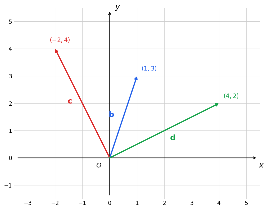
Graphical representation of vectors b, c, and d as directed segments from the origin to the points (1,3), (-2,4), and (4,2)

Example 2

The vectors $\mathbf{b} = \begin{bmatrix} 1 \\ 3 \end{bmatrix}$ , $\mathbf{c} = \begin{bmatrix} -2 \\ 4 \end{bmatrix}$ , and $\mathbf{d} = \begin{bmatrix} 4 \\ 2 \end{bmatrix}$ are represented in the figure above as directed arrows from the origin to the points $(1, 3)$ , $(-2, 4)$ , and $(4, 2)$ respectively. The components of each vector are precisely the coordinates of the arrowhead.

An ordered pair of real numbers can fundamentally represent two distinct concepts: a geometric point or an algebraic vector. Points are fixed locations in the plane; vectors are algebraic quantities that typically represent displacements or shifts. We adopt the following convention to distinguish them.

Remark (Point vs Vector)

A point is denoted by a capital letter with coordinates in parentheses: $A = (a_1, a_2)$ .
A vector is denoted by a bold lower-case letter as a column: $\mathbf{a} = \begin{bmatrix} a_1 \\ a_2 \end{bmatrix}$ .

This distinction is not merely cosmetic. The point $A = (3, 5)$ is a fixed location in the plane. The vector $\mathbf{a} = \begin{bmatrix} 3 \\ 5 \end{bmatrix}$ represents a displacement of $3$ units horizontally and $5$ units vertically. When we draw $\mathbf{a}$ as an arrow from the origin to $A$ , we are anchoring the displacement at a specific starting point, but the displacement itself is independent of where it begins. This will become clearer when we discuss vector addition and translation in subsequent sections.

Example 3

Consider a city grid where the origin is placed at the town hall. The police station sits at the point $P = (2, 3)$ , a fixed location. The instruction “walk $2$ blocks east and $3$ blocks north” is the vector $\mathbf{p} = \begin{bmatrix} 2 \\ 3 \end{bmatrix}$ , a displacement that makes sense from any starting position. If you follow $\mathbf{p}$ from the town hall, you arrive at $P$ . If you follow $\mathbf{p}$ from the library at $(1, 1)$ , you arrive at $(3, 4)$ instead. The vector is the same; the destination changes with the starting point.

Problem 1

Let $\mathbf{u} = \begin{bmatrix} x + 1 \\ 3 \end{bmatrix}$ and $\mathbf{v} = \begin{bmatrix} 4 \\ y - 2 \end{bmatrix}$ . Determine the values of $x$ and $y$ for which $\mathbf{u} = \mathbf{v}$ .

Problem 2

A particle starts at the origin and undergoes two successive displacements: first $\mathbf{p} = \begin{bmatrix} 3 \\ -1 \end{bmatrix}$ , then $\mathbf{q} = \begin{bmatrix} -1 \\ 4 \end{bmatrix}$ . Without defining vector addition formally, determine the coordinates of the particle’s final position by applying each displacement component-wise. What single vector from the origin would land the particle at the same final position?

Magnitude

Given a vector $\mathbf{a} = \begin{bmatrix} a_1 \\ a_2 \end{bmatrix}$ , the directed segment from the origin $O$ to the point $A = (a_1, a_2)$ has a length determined by Pythagoras’ theorem. We define this length as the magnitude of the vector.

Definition 3 (Magnitude)

The magnitude (or norm) of a vector $\mathbf{a} = \begin{bmatrix} a_1 \\ a_2 \end{bmatrix}$ , denoted $|\mathbf{a}|$ , is the non-negative real number given by:

|\mathbf{a}| = \sqrt{a_1^2 + a_2^2}

Example 4

For the vectors from the figure above, we compute:

|\mathbf{b}| = \sqrt{1^2 + 3^2} = \sqrt{10}, \qquad |\mathbf{c}| = \sqrt{(-2)^2 + 4^2} = \sqrt{20}, \qquad |\mathbf{d}| = \sqrt{4^2 + 2^2} = \sqrt{20}.

Observe that $\mathbf{c}$ and $\mathbf{d}$ have different components but equal magnitude. Magnitude alone does not determine a vector.

Vectors with magnitude $1$ are of particular importance.

Definition 4 (Unit Vector)

A vector $\mathbf{u}$ is called a unit vector if $|\mathbf{u}| = 1$ .

Examples include $\begin{bmatrix} 1/\sqrt{2} \\ -1/\sqrt{2} \end{bmatrix}$ and, more generally, $\begin{bmatrix} \cos\theta \\ \sin\theta \end{bmatrix}$ for any angle $\theta$ . The standard unit coordinate vectors are denoted

\mathbf{e}_1 = \begin{bmatrix} 1 \\ 0 \end{bmatrix}, \qquad \mathbf{e}_2 = \begin{bmatrix} 0 \\ 1 \end{bmatrix}.

Every vector in the plane decomposes uniquely in terms of these two: if $\mathbf{a} = \begin{bmatrix} a_1 \\ a_2 \end{bmatrix}$ , then $\mathbf{a} = a_1\mathbf{e}_1 + a_2\mathbf{e}_2$ , as one verifies directly from the definitions. The components of $\mathbf{a}$ are therefore precisely the coefficients of $\mathbf{e}_1$ and $\mathbf{e}_2$ in this decomposition.

Theorem 1 (Zero Vector Magnitude)

Let $\mathbf{a}$ be a vector. Then $|\mathbf{a}| = 0$ if and only if $\mathbf{a} = \mathbf{0}$ .

Proof

Since $a_1^2 \geq 0$ and $a_2^2 \geq 0$ for any real numbers, the sum $a_1^2 + a_2^2 = 0$ implies $a_1 = 0$ and $a_2 = 0$ . Conversely, if $a_1 = a_2 = 0$ , the magnitude is clearly zero.

■

This characterises the zero vector (Definition 2) as the unique vector with zero magnitude. Geometrically, it corresponds to a degenerate segment where the initial and terminal points coincide at the origin. All other vectors are non-zero, possessing a well-defined positive magnitude and a specific direction.

Problem 3

For what values of $t \in \mathbb{R}$ is $\begin{bmatrix} t \\ 1 - t \end{bmatrix}$ a unit vector?

The Vector Space $\mathbb{R}^2$

The primary advantage of vector geometry lies in the algebraic system formed by vectors, which mirrors properties of complex numbers. We define two fundamental operations: addition and scalar multiplication.

Definition 5 (Vector Addition)

Let $\mathbf{a} = \begin{bmatrix} a_1 \\ a_2 \end{bmatrix}$ and $\mathbf{b} = \begin{bmatrix} b_1 \\ b_2 \end{bmatrix}$ be vectors. The sum $\mathbf{a} + \mathbf{b}$ is defined as:

\mathbf{a} + \mathbf{b} = \begin{bmatrix} a_1 + b_1 \\ a_2 + b_2 \end{bmatrix}

The reader who solved Problem 2 has already performed this operation: combining the displacements $\mathbf{p}$ and $\mathbf{q}$ component-wise is precisely vector addition.

Definition 6 (Scalar Multiplication)

Let $\mathbf{a} = \begin{bmatrix} a_1 \\ a_2 \end{bmatrix}$ be a vector and $r \in \mathbb{R}$ a scalar. The scalar multiple $r\mathbf{a}$ is defined as:

r\mathbf{a} = \begin{bmatrix} ra_1 \\ ra_2 \end{bmatrix}

We also define the negative of a vector as $-\mathbf{a} = (-1)\mathbf{a} = \begin{bmatrix} -a_1 \\ -a_2 \end{bmatrix}$ , and vector subtraction as $\mathbf{b} - \mathbf{a} = \mathbf{b} + (-\mathbf{a})$ .

Definition 7 (Linear Combination)

A linear combination of vectors $\mathbf{a}$ and $\mathbf{b}$ is any expression of the form $c\mathbf{a} + d\mathbf{b}$ , where $c, d \in \mathbb{R}$ .

Vector addition, subtraction, and scalar multiples are all special cases: $\mathbf{a} + \mathbf{b} = 1\cdot\mathbf{a} + 1\cdot\mathbf{b}$ , the difference is $1\cdot\mathbf{a} + (-1)\cdot\mathbf{b}$ , and $c\mathbf{a} = c\cdot\mathbf{a} + 0\cdot\mathbf{b}$ . The zero vector itself is the linear combination $0\cdot\mathbf{a} + 0\cdot\mathbf{b}$ .

Example 5

Let $\mathbf{a} = \begin{bmatrix} 3 \\ -1 \end{bmatrix}$ and $\mathbf{b} = \begin{bmatrix} 2 \\ 4 \end{bmatrix}$ . Then:

\mathbf{a} + \mathbf{b} = \begin{bmatrix} 5 \\ 3 \end{bmatrix}, \qquad 3\mathbf{a} = \begin{bmatrix} 9 \\ -3 \end{bmatrix}, \qquad \mathbf{a} - \mathbf{b} = \begin{bmatrix} 1 \\ -5 \end{bmatrix}.

Geometric Interpretation

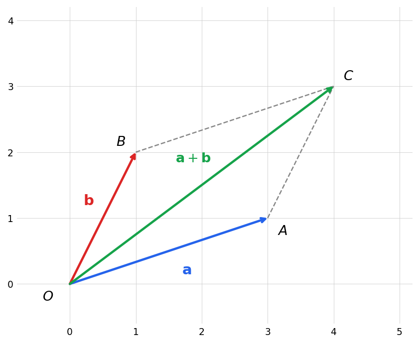
Vector addition adheres to the Parallelogram Law. If vectors $\mathbf{a}$ and $\mathbf{b}$ are represented by directed segments $\overrightarrow{OA}$ and $\overrightarrow{OB}$ , their sum $\mathbf{c} = \mathbf{a} + \mathbf{b}$ corresponds to $\overrightarrow{OC}$ , where $OACB$ forms a parallelogram.

The Parallelogram Law of vector addition

An equivalent description is the head-to-tail rule: place the start of $\mathbf{b}$ at the tip of $\mathbf{a}$ ; the endpoint of $\mathbf{b}$ then lands at the tip of $\mathbf{a} + \mathbf{b}$ . Traversing $\mathbf{a}$ then $\mathbf{b}$ , or $\mathbf{b}$ then $\mathbf{a}$ , traces opposite sides of the same parallelogram, confirming commutativity (Theorem 2, Property 1) geometrically.

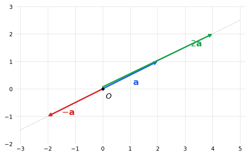
Scalar multiplication $r\mathbf{a}$ corresponds to scaling the length of the vector by a factor of $|r|$ . If $r > 0$ , the direction remains unchanged; if $r < 0$ , the direction is reversed. If $r = 0$ , the result is the zero vector (Definition 2).

Definition 8 (Vector Space

\mathbb{R}^2

)

The collection of all vectors in the plane, together with the operations of vector addition and scalar multiplication, is denoted $\mathbb{R}^2$ and is called the vector space of the plane.

Remark

These definitions extend naturally to any number of components. A vector in $\mathbb{R}^3$ has three components $\begin{bmatrix} a_1 \\ a_2 \\ a_3 \end{bmatrix}$ , and addition and scalar multiplication proceed component-wise as before. More generally, a vector in $\mathbb{R}^n$ is an ordered $n$ -tuple of real numbers, and the same axioms continue to hold. When writing vectors with many components inline, we sometimes use the row shorthand $\mathbf{v} = (v_1, v_2, v_3)$ ; this is still understood as a column vector temporarily lying on its side to save space, not as a row vector.

The algebraic structure of $\mathbb{R}^2$ is governed by the following fundamental properties.

Theorem 2 (Properties of

\mathbb{R}^2

)

Let $\mathbf{a}, \mathbf{b}, \mathbf{c}$ be vectors in $\mathbb{R}^2$ and let $r, s$ be scalars. Then:

$\mathbf{a} + \mathbf{b} = \mathbf{b} + \mathbf{a}$ (Commutativity)
$(\mathbf{a} + \mathbf{b}) + \mathbf{c} = \mathbf{a} + (\mathbf{b} + \mathbf{c})$ (Associativity)
There exists a unique vector $\mathbf{0}$ such that $\mathbf{a} + \mathbf{0} = \mathbf{a}$ . (Additive Identity)
For every $\mathbf{a}$ , there exists a unique vector $-\mathbf{a}$ such that $\mathbf{a} + (-\mathbf{a}) = \mathbf{0}$ . (Additive Inverse)
$(rs)\mathbf{a} = r(s\mathbf{a})$
$(r + s)\mathbf{a} = r\mathbf{a} + s\mathbf{a}$
$r(\mathbf{a} + \mathbf{b}) = r\mathbf{a} + r\mathbf{b}$
$1\mathbf{a} = \mathbf{a}$

The proof follows directly from the properties of real numbers applied to the components. For example, $\mathbf{a} + \mathbf{b} = \begin{bmatrix} a_1 + b_1 \\ a_2 + b_2 \end{bmatrix} = \begin{bmatrix} b_1 + a_1 \\ b_2 + a_2 \end{bmatrix} = \mathbf{b} + \mathbf{a}$ .

Remark

The correspondence between complex numbers and vectors is notable. Identifying $\mathbf{a} = \begin{bmatrix} a_1 \\ a_2 \end{bmatrix}$ with $z = a_1 + ia_2$ , vector addition corresponds to complex addition, and scalar multiplication corresponds to multiplying a complex number by a real number. However, unlike complex numbers, $\mathbb{R}^2$ does not inherently possess a vector-by-vector multiplication operation in this context.

We now demonstrate the power of these axioms by proving algebraic theorems in two ways: first using components (concrete), and second using only the axioms (abstract). This dual approach highlights that the results hold for any system satisfying the properties of Theorem 2, not just $\mathbb{R}^2$ .

Theorem 3 (Zero Product Law)

Let $\mathbf{a}$ be a vector and $r$ a scalar. Then $r\mathbf{a} = \mathbf{0}$ if and only if $r = 0$ or $\mathbf{a} = \mathbf{0}$ .

Proof 1 (Components)

Let $\mathbf{a} = \begin{bmatrix} a_1 \\ a_2 \end{bmatrix}$ . Then $r\mathbf{a} = \begin{bmatrix} ra_1 \\ ra_2 \end{bmatrix}$ .

If $r = 0$ , then $r\mathbf{a} = \begin{bmatrix} 0 \\ 0 \end{bmatrix} = \mathbf{0}$ . If $\mathbf{a} = \mathbf{0}$ , then $a_1 = a_2 = 0$ , so $r\mathbf{a} = \begin{bmatrix} 0 \\ 0 \end{bmatrix} = \mathbf{0}$ .

Conversely, suppose $r\mathbf{a} = \mathbf{0}$ . Then $ra_1 = 0$ and $ra_2 = 0$ . If $r \neq 0$ , we must have $a_1 = 0$ and $a_2 = 0$ , so $\mathbf{a} = \mathbf{0}$ .

■

Proof 2 (Axiomatic)

We use the properties from Theorem 2.

To show $0\mathbf{a} = \mathbf{0}$ :

0\mathbf{a} = (0 + 0)\mathbf{a} \overset{(6)}{=} 0\mathbf{a} + 0\mathbf{a}.

Adding $-(0\mathbf{a})$ to both sides gives $\mathbf{0} = 0\mathbf{a}$ .

To show $r\mathbf{0} = \mathbf{0}$ :

r\mathbf{0} = r(\mathbf{0} + \mathbf{0}) \overset{(7)}{=} r\mathbf{0} + r\mathbf{0}.

Adding $-(r\mathbf{0})$ to both sides gives $\mathbf{0} = r\mathbf{0}$ .

Conversely, suppose $r\mathbf{a} = \mathbf{0}$ with $r \neq 0$ . Then $1/r$ exists and

\mathbf{a} \overset{(8)}{=} 1\mathbf{a} = \left(\tfrac{1}{r} \cdot r\right)\mathbf{a} \overset{(5)}{=} \tfrac{1}{r}(r\mathbf{a}) = \tfrac{1}{r}\mathbf{0} = \mathbf{0}.

■

Theorem 4 (Negative Scalars)

Let $\mathbf{a}$ be a vector and $r$ a scalar. Then:

(-r)\mathbf{a} = r(-\mathbf{a}) = -(r\mathbf{a})

Proof 1 (Components)

Let $\mathbf{a} = \begin{bmatrix} a_1 \\ a_2 \end{bmatrix}$ . Then:

(-r)\mathbf{a} = \begin{bmatrix} -ra_1 \\ -ra_2 \end{bmatrix}, \qquad r(-\mathbf{a}) = r\begin{bmatrix} -a_1 \\ -a_2 \end{bmatrix} = \begin{bmatrix} -ra_1 \\ -ra_2 \end{bmatrix}, \qquad -(r\mathbf{a}) = -\begin{bmatrix} ra_1 \\ ra_2 \end{bmatrix} = \begin{bmatrix} -ra_1 \\ -ra_2 \end{bmatrix}.

All three expressions yield identical components.

■

Proof 2 (Axiomatic)

The vector $-(r\mathbf{a})$ is defined as the unique additive inverse of $r\mathbf{a}$ . It suffices to show that both $(-r)\mathbf{a}$ and $r(-\mathbf{a})$ act as inverses of $r\mathbf{a}$ .

For $(-r)\mathbf{a}$ :

r\mathbf{a} + (-r)\mathbf{a} \overset{(6)}{=} (r + (-r))\mathbf{a} = 0\mathbf{a} = \mathbf{0}.

For $r(-\mathbf{a})$ :

r\mathbf{a} + r(-\mathbf{a}) \overset{(7)}{=} r(\mathbf{a} + (-\mathbf{a})) = r\mathbf{0} = \mathbf{0}.

Since additive inverses are unique (Property 4), $(-r)\mathbf{a} = r(-\mathbf{a}) = -(r\mathbf{a})$ .

■

Problem 4

Using only the properties from Theorem 2, prove that $\mathbf{a} + \mathbf{b} = \mathbf{a} + \mathbf{c}$ implies $\mathbf{b} = \mathbf{c}$ (the cancellation law).

Linear Independence

While $\mathbf{e}_1$ and $\mathbf{e}_2$ generate the plane, they also satisfy a property of non-redundancy: neither is a scalar multiple of the other. If $\mathbf{e}_1 = r\mathbf{e}_2$ , then $\begin{bmatrix} 1 \\ 0 \end{bmatrix} = \begin{bmatrix} 0 \\ r \end{bmatrix}$ , implying $1 = 0$ , a contradiction. This concept is formalised as linear independence.

Definition 9 (Linear Dependence and Independence)

Two vectors $\mathbf{a}$ and $\mathbf{b}$ in $\mathbb{R}^2$ are said to be linearly dependent if one is a scalar multiple of the other. That is, either $\mathbf{a} = r\mathbf{b}$ or $\mathbf{b} = s\mathbf{a}$ for some scalars $r, s$ .

If neither vector is a scalar multiple of the other, they are said to be linearly independent.

Remark

If $\mathbf{a} = \mathbf{0}$ , then $\mathbf{a} = 0\mathbf{b}$ , making the pair linearly dependent. Similarly, any vector is linearly dependent with itself. Thus, linear independence is a property relevant to distinct, non-zero vectors.

Geometrically, two non-zero vectors are linearly dependent if and only if they are collinear with the origin; that is, the directed segments $\overrightarrow{OA}$ and $\overrightarrow{OB}$ lie on the same straight line passing through $O$ .

This has a striking consequence for linear combinations. If $\mathbf{a}$ and $\mathbf{b}$ are linearly dependent and non-zero, every combination $c\mathbf{a} + d\mathbf{b}$ is a scalar multiple of $\mathbf{a}$ (since $\mathbf{b}$ itself is), so the combinations fill only the line through the origin in the direction of $\mathbf{a}$ . If $\mathbf{a}$ and $\mathbf{b}$ are linearly independent, the opposite holds: for any target vector $\mathbf{t} = \begin{bmatrix} t_1 \\ t_2 \end{bmatrix}$ , the system $c\mathbf{a} + d\mathbf{b} = \mathbf{t}$ amounts to two equations in two unknowns, and when $a_1 b_2 - a_2 b_1 \neq 0$ this system always has a unique solution. The combinations therefore fill the entire plane $\mathbb{R}^2$ . Determining which situation holds is a question of fundamental importance.

Theorem 5 (Determinant Criterion for Dependence)

Let $\mathbf{a} = \begin{bmatrix} a_1 \\ a_2 \end{bmatrix}$ and $\mathbf{b} = \begin{bmatrix} b_1 \\ b_2 \end{bmatrix}$ . The vectors $\mathbf{a}$ and $\mathbf{b}$ are linearly dependent if and only if

a_1 b_2 - a_2 b_1 = 0.

Proof

Suppose $a_1 b_2 - a_2 b_1 = 0$ . If $\mathbf{a} = \mathbf{0}$ , the vectors are dependent. Assume $\mathbf{a} \neq \mathbf{0}$ ; then at least one component, say $a_1$ , is non-zero. From $a_1 b_2 = a_2 b_1$ , we have $b_2 = \frac{a_2}{a_1}b_1$ . We can express $\mathbf{b}$ as:

\mathbf{b} = \begin{bmatrix} b_1 \\ b_2 \end{bmatrix} = \begin{bmatrix} b_1 \\ \frac{a_2}{a_1}b_1 \end{bmatrix} = \frac{b_1}{a_1} \begin{bmatrix} a_1 \\ a_2 \end{bmatrix} = \frac{b_1}{a_1}\,\mathbf{a}.

Thus $\mathbf{b}$ is a scalar multiple of $\mathbf{a}$ . A similar argument holds if $a_2 \neq 0$ .

Conversely, suppose $\mathbf{a}$ and $\mathbf{b}$ are linearly dependent. If $\mathbf{a} = r\mathbf{b}$ , then $a_1 = rb_1$ and $a_2 = rb_2$ . Substituting:

a_1 b_2 - a_2 b_1 = (rb_1)b_2 - (rb_2)b_1 = r(b_1 b_2 - b_2 b_1) = 0.

The same result follows if $\mathbf{b} = s\mathbf{a}$ .

■

The expression $a_1 b_2 - a_2 b_1$ is called the determinant of the pair of vectors. It plays a role analogous to the discriminant in quadratic equations, providing a purely algebraic test for a geometric property. We will see more of this in subsequent notes.

Example 6

Consider $\mathbf{a} = \begin{bmatrix} 2 \\ 4 \end{bmatrix}$ and $\mathbf{b} = \begin{bmatrix} 1 \\ 2 \end{bmatrix}$ . The determinant is $2 \cdot 2 - 4 \cdot 1 = 0$ , so the pair is linearly dependent. Indeed, $\mathbf{a} = 2\mathbf{b}$ .

Now consider $\mathbf{a} = \begin{bmatrix} 3 \\ 1 \end{bmatrix}$ and $\mathbf{b} = \begin{bmatrix} 1 \\ 2 \end{bmatrix}$ . The determinant is $3 \cdot 2 - 1 \cdot 1 = 5 \neq 0$ , so the pair is linearly independent: neither is a scalar multiple of the other.

We may also characterise linear dependence through linear combinations yielding the zero vector.

Theorem 6 (Algebraic Criterion for Dependence)

Two vectors $\mathbf{a}$ and $\mathbf{b}$ are linearly dependent if and only if there exist scalars $r$ and $s$ , not both zero, such that

r\mathbf{a} + s\mathbf{b} = \mathbf{0}.

Proof

Suppose such scalars exist. Without loss of generality, assume $r \neq 0$ . Then we can rearrange:

r\mathbf{a} = -s\mathbf{b} \implies \mathbf{a} = \left(-\frac{s}{r}\right)\mathbf{b}.

Thus $\mathbf{a}$ is a scalar multiple of $\mathbf{b}$ , implying dependence.

Conversely, if $\mathbf{a}$ and $\mathbf{b}$ are dependent, then either $\mathbf{a} = k\mathbf{b}$ or $\mathbf{b} = k\mathbf{a}$ . In the first case, $1\cdot\mathbf{a} + (-k)\mathbf{b} = \mathbf{0}$ (where $r = 1 \neq 0$ ). In the second, $(-k)\mathbf{a} + 1\cdot\mathbf{b} = \mathbf{0}$ (where $s = 1 \neq 0$ ).

■

We summarise these findings in two equivalent statements, distinguishing the dependent and independent cases.

Theorem 7 (Conditions for Linear Dependence)

Let $\mathbf{a} = \begin{bmatrix} a_1 \\ a_2 \end{bmatrix}$ and $\mathbf{b} = \begin{bmatrix} b_1 \\ b_2 \end{bmatrix}$ be vectors in $\mathbb{R}^2$ . The following statements are equivalent:

$\mathbf{a}$ and $\mathbf{b}$ are linearly dependent.
The points $O = (0,0)$ , $A = (a_1, a_2)$ , and $B = (b_1, b_2)$ are collinear.
$a_1 b_2 - a_2 b_1 = 0$ .
There exist scalars $r, s$ , not both zero, such that $r\mathbf{a} + s\mathbf{b} = \mathbf{0}$ .

Theorem 8 (Conditions for Linear Independence)

Let $\mathbf{a} = \begin{bmatrix} a_1 \\ a_2 \end{bmatrix}$ and $\mathbf{b} = \begin{bmatrix} b_1 \\ b_2 \end{bmatrix}$ be vectors in $\mathbb{R}^2$ . The following statements are equivalent:

$\mathbf{a}$ and $\mathbf{b}$ are linearly independent.
$\mathbf{a}$ and $\mathbf{b}$ are non-zero, and the points $O$ , $A$ , $B$ are distinct and not collinear.
$a_1 b_2 - a_2 b_1 \neq 0$ .
The equation $r\mathbf{a} + s\mathbf{b} = \mathbf{0}$ implies $r = 0$ and $s = 0$ .

Remark

One should observe the distinction between the two types of proofs presented in this chapter.

Component-based proofs (e.g., Theorem 2, Theorem 5) rely on the explicit definition of a vector as an ordered pair of numbers. These are specific to $\mathbb{R}^2$ .
Axiomatic proofs (e.g., Theorem 3, Theorem 6) rely only on the algebraic properties of vector addition and scalar multiplication. These proofs are more powerful as they apply to any vector space, regardless of dimension or the nature of the vectors involved.

Problem 5

Let $\mathbf{a} = \begin{bmatrix} 2 \\ -3 \end{bmatrix}$ and $\mathbf{b} = \begin{bmatrix} -4 \\ t \end{bmatrix}$ . Determine the value of $t$ for which $\mathbf{a}$ and $\mathbf{b}$ are linearly dependent. For this value of $t$ , express $\mathbf{b}$ as a scalar multiple of $\mathbf{a}$ .

Video

Lesson assets

Vectors

Vectors in the Plane

Visualisation

Magnitude

The Vector Space R2\mathbb{R}^2R2

Geometric Interpretation

Linear Independence

The Vector Space $\mathbb{R}^2$