
Predicates, Numbers, and Sets
Predicate Logic
We realise that propositional logic is not enough. If we know that “all men are mortal” and “Socrates is a man”, it ought to follow that “Socrates is mortal.” But propositional logic cannot reach this conclusion: it treats each sentence as an indivisible whole and cannot look inside to see the relationship between the object (Socrates), the property (being a man), and the consequence (being mortal).
To see the problem more concretely, consider the following mathematical argument:
Every prime number greater than is odd. The number is a prime number greater than . Therefore, is odd.
This looks like a straightforward application of modus ponens (Lesson 1). Yet propositional logic cannot carry it out: there is no way to symbolise “Every prime number greater than is odd” as a conditional whose premise is “The number is a prime number greater than .” The first sentence speaks about all primes; the second speaks about a specific number. Propositional logic has no mechanism to connect the two.
What is missing is the ability to distinguish the object of our speech from the description we make about it. To overcome this, we introduce predicate logic, which allows us to reason about objects and their properties.
Variables and Predicates
Recall that a variable is a symbol standing in for an object that has not yet been specified, and a term is a symbol denoting an object (Lesson 1). Specific terms such as the natural number or the constant are called constants; variables are terms whose value has not been determined. A term on its own does not form a complete sentence and has no truth value.
We can attach a description to a variable: write to say ” is a man”, or to say ” is a number larger than .” These expressions are not propositions (Definition 1), because their truth value depends on what actually is.
Let be variable symbols. We say is an -ary predicate if replacing each variable with a term results in a proposition that has a truth value.
- A -ary (monadic) predicate describes a property, e.g., .
- A -ary (dyadic) predicate describes a relation between two terms, e.g., .
- An -ary predicate describes a relation among terms.
If is the monadic predicate for being prime and is a term, then is the proposition ” is prime.” If is the dyadic predicate for “is greater than”, then is the proposition ” is greater than .” These are the atomic propositions of first-order logic.
Let denote , where the variables range over the integers. Then is since ; is since ; and is still a predicate, since can be or depending on the values of and .
A predicate’s variables take values in a domain , called the universe of discourse. In the previous example, is the integers. Once values from are substituted, the predicate becomes a proposition with truth value or . Hence the logical connectives from Lesson 1 apply directly.
Let denote . Then the following are :
And the following are :
More generally, we can build new predicates out of old ones using connectives. Expressions constructed from predicates and logical connectives that still contain free variables are called propositional functions.
Using as above, the following are propositional functions:
is a predicate in two variables; is a predicate in one variable (since is already a proposition).
Problem 17
Consider the expressions , , and . Which of these are propositions (Definition 1) and which are predicates? For each predicate, give one substitution that makes it and one that makes it .
Aristotle developed a limited form of predicate logic through his theory of syllogisms. The modern version was independently developed by Frege and Peirce between the 19th and 20th centuries, roughly 2000 years later, mirroring the timeline of propositional logic itself (Lesson 1). Predicate logic (also called first-order logic) is now the standard language for mathematical statements and is equally fundamental in computer science, appearing in database queries, logic programming (Prolog), automated theorem proving, software verification, and symbolic AI. Some mathematicians, notably Hilbert, hoped it would be a complete system for all of mathematics, but Gödel’s incompleteness theorem showed otherwise: no fixed set of axioms can prove all true mathematical statements.
Sets and Numbers
We have been throwing around numbers and their collections somewhat loosely. In Lesson 1, Example 1 asserted "" and Example 1 item 3 stated “For any real number , ”, while the truth tables themselves are indexed by rows we count with integers. Earlier we had hints to specific collections of numbers. It is time to properly introduce them.
Fundamental to mathematics is the notion of a set. We will study sets in great detail in later lessons, but from this point onwards you will find them in every chapter of this textbook, so we take some time to think about them now. We will not treat sets formally at this stage; for now, the following definition will suffice.
A set is a collection of objects. The objects in the set are called elements of the set. If is a set and is an object, then we write to denote the assertion that is an element of .
The sets of concern to us first and foremost are the number sets: sets whose elements are particular types of number. At this introductory level, many details will be temporarily swept under the rug; we will work at a level of precision which is appropriate for our current stage, but still allows us to develop a reasonable amount of intuition.
Later on, if time permits, we plan to cover the construction of the number systems from first principles. For now, we start with the simple build-up.
Numbers and Magnitude
The study of mathematics is built upon the study of increasing and decreasing quantities, or magnitudes, sometimes referred to as the science of quantity.
From the fruit that a person purchases at a store, to the measurement of vast interstellar distances, the concept of quantity is ubiquitous. However, we cannot quantify or determine a specific amount except by comparing it to a similar magnitude of the same kind. For instance, when enumerating fruit, we might regard the collection as a single total or distinguish them by category (apples, pears, bananas). To formalise this comparison, we require a standard.
A unit is a chosen reference magnitude of a particular species, fixed as the standard for comparison within that species.
A unit is the basic reference “one” for a kind of quantity. For continuous quantities it is not a smallest possible part, because we may subdivide further. If you change the unit, the numerical measure changes, but the quantity being measured remains the same.
A measure is the number assigned to a magnitude relative to a chosen unit of the same species. If is a magnitude and is the chosen unit, its measure is the number such that .
In this measurement frame (used for ), a number records the signed comparison of a magnitude with a chosen unit of the same species. The complex numbers will later extend this arithmetic framework geometrically.
Stand at the edge of a beach and draw a small square in the sand. Everything inside that square is our amount of sand. Before we start, we choose a unit: one handful. Now scoop the sand out, one handful at a time, saying the numbers out loud as you go. The last number you say is the measure of that sand in handfuls.
If you switch to a bigger scoop and repeat, you will finish sooner and stop at a smaller number. If you switch to a tiny spoon, you will take longer and stop at a bigger number. The sand did not change. Only the unit changed, so the number you report changed with it.
Write the chosen unit as and the magnitude as . The measured number is with . This is exactly the model we use on the number line: once and the unit length are fixed, each point gets the signed measure of its displacement from in that unit.
Problem 17A (Unit and Measure Check)
Suppose a rope has measure when the unit is metre.
- What is its measure if the unit is changed to metre?
- What is its measure if the unit is changed to metres?
- Explain, in one sentence, why these two answers do not describe two different ropes.
The Number Line
In order to define the number sets, we will need three things: an infinite line, a fixed point on this line, and a fixed unit of length.
So here we go. Here is an infinite line:

The arrows indicate that it is supposed to extend in both directions without end. The points on the line will represent numbers (specifically, real numbers, a misleading term that will be defined later).
Now let us fix a point on this line, and label it :

This point represents the number zero; it is the point against which all other numbers will be measured. Numbers to the left of on the line are said to be negative, and those to the right are positive; itself is neither positive nor negative.
Finally, let us fix a unit of length:

This unit of length turns position into measure: each point is assigned a signed number telling how many unit lengths it lies from .
The above infinite line, together with its fixed zero point and fixed unit length, constitute the (real) number line.
We will use the number line to construct the principal number sets of interest to us: the set of natural numbers, the set of integers, the set of rational numbers, and the set of real numbers. Each of these sets has a different character and is used for different purposes, as we will see throughout this course.
Natural Numbers ()
The natural numbers are the numbers used for counting. They are the answers to questions of the form “how many”: I have three uncles, three guinea pigs, and zero cats.
The numbers we use for counting objects, such as , and so on, are called the natural numbers. This family of numbers is generated by starting at and successively adding one unit. We use the symbol as a shorthand to refer to all natural numbers.
The natural numbers are represented by the points on the number line which can be obtained by starting at and moving right by the unit length any number of times:

In more familiar terms, they are the non-negative whole numbers. The notation means that is a natural number.
There is an important aspect of this topic we will not study now: the representation of numbers in different bases. In English, the Arabic numerals are used as the ten digits , forming the most popular system (base ). Other bases exist and are fundamental in computing (base , base ), but their treatment is deferred to a later chapter.
Integers ()
Addition combines magnitudes; its inverse takes them away. This inverse operation is called subtraction, denoted by the symbol . Formally, subtraction is the inverse of addition, meaning the operation undoes the effect of , and vice versa. This relationship is expressed by:
The symbols and act as signs that instruct how a quantity is to be treated. A preceding means “to be added”; a preceding means “to be subtracted.” The expression means “to the quantity , add the quantity .”
We can also view subtraction as finding a “missing addend.”
For numbers and , the difference is the unique number that one must add to to obtain . We write to mean “implies”, marking a valid step from one statement to the next:
Our definition of subtraction has so far assumed that is larger than . What about ? Using Definition 22, we seek a number such that . No such number exists among the natural numbers.
Algebra is the general theory of these operations; we establish laws and follow them. When results like cannot be interpreted with our current numbers, they force us to invent new concepts that are consistent with our laws.
Mechanically, calculating means starting at and applying the predecessor action five times:
A step to the left from takes us off the natural number line. To resolve this, we must extend our system. A step of from lands on a point we call negative one, or . A further step lands on .
A negative number, denoted , is the number that results from subtracting a positive number from zero:
With this, we can complete our calculation: .
By extending our number line to include these new negative numbers, along with zero and the natural numbers, we form a more complete system.
The system of numbers formed by combining the natural numbers (), their negative counterparts, and zero is called the integers. This collection of whole numbers, stretching infinitely in both positive and negative directions, is denoted by the symbol :
The integers can be used for measuring the difference between two natural numbers. For example, suppose you have five apples and five bananas. Another person, also holding apples and bananas, wishes to trade. After the exchange, you have seven apples and only one banana. Thus you have two more apples and four fewer bananas.
Since an increment in quantity can be represented by moving to the right on the number line by the unit length, a decrement in quantity can therefore be represented by moving to the left by the unit length. Doing so gives rise to the integers:

The notation means that is an integer.
Rational Numbers ()
Just as subtraction forced us beyond the natural numbers, division now forces us beyond the integers. But before we can discuss division, we need its prerequisite.
Multiplication of a number by a natural number is the repeated addition of exactly times:
For numbers and (where is not zero), the quotient is the unique number that one must multiply by to obtain :
In the expression , is the dividend and is the divisor.
Another standard notation for division is the fraction bar, where is written as . This notation is familiar from arithmetic, where represents of the -th parts of a unit. We can see that these two ideas are the same: if we take copies of the quantity , we have , which by the arithmetical definition is . Since this matches our algebraic definition (Definition 26), the notations are equivalent and can be used interchangeably.
In this chapter, , , and all denote multiplication. We use only when repeated addition or counting factors is being emphasised.
The motivation for the next number system is that the result of dividing one integer by another is not necessarily another integer. However, the result is sometimes an integer; for example, six apples can be divided between three people, and each person receives an integral number of apples.
This makes division interesting: how can we measure the failure of one integer’s divisibility by another? How can we deduce when one integer is divisible by another? What is the structure of the set of integers when viewed through the lens of division? This set of questions is so important it spans a large portion of the second half of this course, in something called number theory.
But for now, we simply need a system of numbers that can express the result of any division (except by zero). Bored of eating apples and bananas, suppose you buy a pizza which is divided into eight slices. A friend and you decide to share it. You eat three slices and your friend eats five. Unfortunately, we cannot represent the proportion of the pizza each of you has eaten using natural numbers or integers. However, we are not far off: we can count the number of equal parts the pizza was split into, and of those parts, we can count how many we had. On the number line, this is represented by splitting the unit line segment from to into eight equal pieces, and proceeding from there. This kind of procedure gives rise to the rational numbers.
The rational numbers are represented by the points on the number line which can be obtained by dividing any of the unit line segments between integers into an equal number of parts. The rational numbers are those of the form , where and are integers and . We denote this collection by .

The notation means that is a rational number.
Problem 18
Why must in Definition 27? Using Definitions 25 and 26, suppose and .
The rational numbers are a very important example of a type of algebraic structure known as a field. We will define this term precisely later. They are particularly central to algebraic number theory and algebraic geometry, subjects we will encounter later.
Real Numbers ()
Quantity and change can be measured in the abstract using real numbers.
The real numbers are the points on the number line. We write for the collection of all real numbers; thus, the notation means that is a real number.
The real numbers are central to real analysis, a branch of mathematics introduced later in this course. They turn the rationals into a continuum by “filling in the gaps”: they have the property of completeness, meaning that if a quantity can be approximated with arbitrary precision by real numbers, then that quantity is itself a real number. We will state a fully formal definition later.
We can define the basic arithmetic operations (addition, subtraction, multiplication and division) on the real numbers, and a notion of ordering, in terms of the infinite number line.
Ordering. A real number is less than a real number , written , if lies to the left of on the number line. The usual conventions for the symbols apply: means that either or .
Addition. Suppose we want to add a real number to a real number . We translate by units to the right; if then this amounts to translating by an equivalent number of units to the left. Concretely, take two copies of the number line, one above the other, with the same choice of unit length. Move the of the lower number line beneath the point of the upper number line. Then is the point on the upper number line lying above the point of the lower number line.
Multiplication. Suppose we want to multiply a real number by a real number . We scale the number line, and perhaps reflect it. Concretely, take two copies of the number line, one above the other. Align the points on both number lines, and stretch the lower number line evenly until the point on the lower number line is below the point on the upper number line (if , the number line must be reflected for this to work). Then is the point on the upper number line lying above on the lower number line.
Real numbers can be constructed rigorously from set theory and about a semester of mathematics. We will accept their existence and properties as axioms for now. If time allows, we plan to properly construct the number systems later. The interested reader may consult constructions via Dedekind cuts or Cauchy sequences.
The real numbers satisfy a collection of axioms that characterise them completely. We state these now for reference; their consequences will be explored throughout the course.
Terms such as “field”, “totally ordered field”, “least upper bound”, and “complete” are signposts for structure that we will define rigorously later. In this chapter, treat (A1)-(A11) as the operational rules for calculation and proof.
(A1) Addition commutes: for all .
(A2) Addition is associative: for all .
(A3) Zero is the additive identity: for all .
(A4) Additive inverses: for each there exists such that .
(A5) Multiplication commutes: for all .
(A6) Multiplication is associative: for all .
(A7) One is the multiplicative identity: for all .
(A8) Multiplicative inverses for nonzero elements: for each there exists such that .
(A9) Distributive properties: and for all .
(A10) Totally ordered field: for :
- (i) Antisymmetry: if and then .
- (ii) Transitivity: if and then .
- (iii) Totality: or .
(A11) Least upper bound property: every nonempty subset of that has an upper bound has a least upper bound. This makes the real numbers complete.
An axiom is a basic belief which cannot be further reduced in the conversation at hand. The axioms (A1)–(A9) make a field, just as is. Axiom (A10) gives it an ordering. Axiom (A11) is what separates from : the rationals satisfy (A1)–(A10) but not (A11).
Apparent obvious facts about numbers require the axioms stated above, and the proofs are worth seeing once: they practise reasoning from first principles and build a toolkit for the chapters ahead.
Uniqueness of zero. Axiom (A3) says that is an additive identity. The following argument shows it is the only one. Suppose for some number . Then
All four properties (A1)–(A4) were needed to justify what amounts to “subtracting from both sides.” A similar argument shows that additive inverses are unique: if then .
Multiplication by zero. Why is ? The number appears only in (A3) and (A4), which concern addition. Without (A9), the axioms say nothing about multiplying by . Since by (A3), distributivity gives
Adding to both sides yields .
The sign rules. Why is the product of two negative numbers positive? This is not a convention; (A1)–(A9) force it. First, :
so is the additive inverse of . With this in hand:
Adding to both sides: . The product of two negative numbers is positive not because we decided it should be, but because (A1)–(A9) leave no alternative.
The zero-product property. If and , then :
by (A6), (A8), and (A7) in turn. Equivalently: if then or . This is the workhorse behind solving polynomial equations by factoring. If , then or , so or . The factorisation is itself a triple application of (A9):
Ordering and squares. The phrase “totally ordered field” in (A10) bundles in two requirements linking the ordering to arithmetic: if then for all ; and if then . Together with the sign rules these yield: if and then , since and .
In particular, whenever , whether is positive or negative. Since and (if then for every , collapsing the number system to a single element), we obtain .
Problem 19
What is wrong with the following “proof”? Let . Then
Problem 20
Prove the following, using only the axioms (A1)–(A9). Write for (axiom A8).
(i) , if .
(ii) , if .
(iii) , if . Hint: remember the defining property of .
(iv) , if .
(v) , if .
(vi) If , then if and only if . Also determine when .
When we ask you to “prove” something in the exercises above, we mean: use the algebraic rules and logical equivalences from Lessons 1 and 1a to show, step by step, that one expression can be transformed into another. Formal proof techniques (contradiction, contrapositive, induction) will be introduced later.
Irrational Numbers
Before we can talk about irrational numbers, we should say what they are.
An irrational number is a real number that is not rational.
Unlike , , , and , there is no standard single letter denoting the irrational numbers. However, once we develop the language of sets more fully, we will be able to write the collection of irrational numbers as (read: “the reals set minus the rationals”).
That such numbers exist at all is not obvious. Consider an isosceles right-angled triangle with both shorter sides of length :
By the Pythagorean theorem, the hypotenuse has length . This is a perfectly concrete geometric magnitude: it is the distance between two corners of a unit square. Yet is not rational. There is no fraction with and that equals exactly.
The discovery of irrational numbers is traditionally attributed to the Pythagorean school (circa 5th century BC). The Pythagoreans believed that all magnitudes could be expressed as ratios of whole numbers. The realisation that the diagonal of a unit square cannot be so expressed is said to have caused a genuine intellectual crisis. According to legend, the member who disclosed this fact, Hippasus of Metapontum, was drowned at sea for his trouble.
Proving that a real number is irrational is not particularly easy, in general. The classical proof that proceeds by contradiction and is one of the most celebrated arguments in all of mathematics. We will carry out this proof later. For now, the interested reader may consult the proof that is irrational. Similar arguments establish the irrationality of , , and in fact for any natural number that is not a perfect square.
Other important irrational numbers arise throughout mathematics: (the ratio of a circle’s circumference to its diameter) and (the base of the natural logarithm) are both irrational, though their proofs require substantially more machinery.
We can use the irrationality of to observe something about how rational and irrational numbers interact under multiplication.
Let . Then and are both irrational, yet , which is rational (Definition 27). The fraction arithmetic established in Problem 20 applies to this number. So the product of two irrational numbers can be rational.
Problem 21
Let be a rational number and let be an irrational number. Prove that it is possible that be rational, and it is possible that be irrational.
Complex Numbers ()
We have seen that multiplication by real numbers corresponds with scaling and reflection of the number line: scaling alone when the multiplicand is positive, and scaling with reflection when it is negative. We could alternatively interpret this reflection as a rotation by half a turn, since the effect on the number line is the same.
You might then wonder what happens if we rotate by arbitrary angles, rather than only half turns. What we end up with is a plane of numbers, not merely a line. Moreover, the rules that we expect arithmetic operations to satisfy still hold: addition corresponds with translation, and multiplication corresponds with scaling and rotation. This resulting number system is that of the complex numbers.
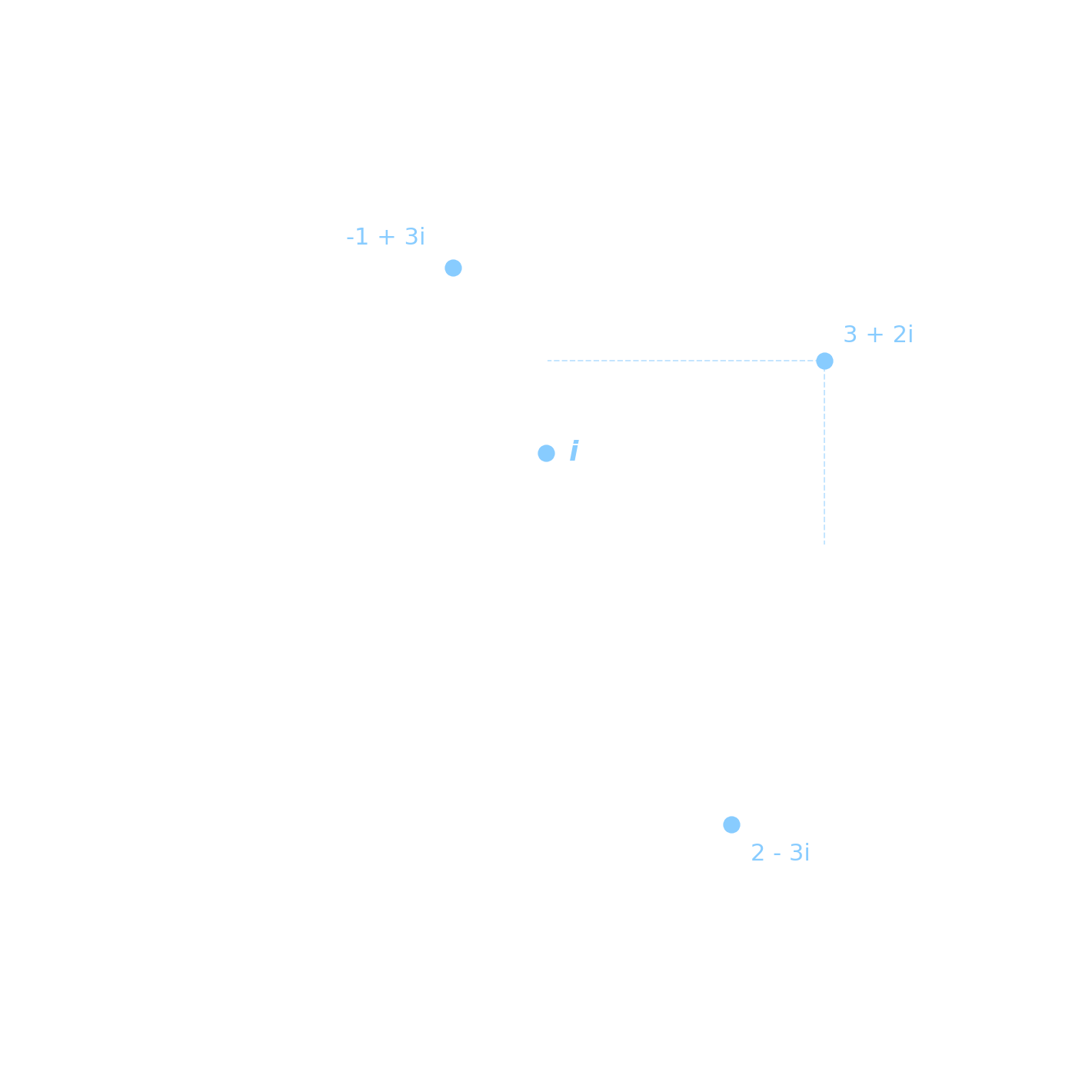
The complex numbers are those obtained from the non-negative real numbers upon rotation by any angle about the point . We write for the collection of all complex numbers; thus, the notation means that is a complex number.
There is a particularly important complex number, , which is the point in the complex plane exactly one unit above :
Multiplication by has the effect of rotating the plane by a quarter turn anticlockwise. In particular, we have
The complex numbers have the astonishing property that square roots of all complex numbers exist, including all the real numbers.
Every complex number can be written in the form , where . This number corresponds with the point on the complex plane obtained by moving units to the right and units up, reversing directions as usual if or is negative. Arithmetic on the complex numbers works just as with the real numbers; in particular, using the fact that , we obtain
We will discuss complex numbers further in the portion of this course on polynomials.
Polynomials
Each of the number sets introduced above comes equipped with nicely behaving notions of addition and multiplication. Polynomials are built from these two operations.
Let or . A (univariate) polynomial over in the indeterminate is an expression of the form
where and each . The numbers are called the coefficients of the polynomial. If not all coefficients are zero, the largest value of for which is called the degree of the polynomial. By convention, the degree of the polynomial is , indicating that has no highest nonzero power term.
Polynomials of degree and are respectively called linear, quadratic, cubic, quartic and quintic polynomials.
The following expressions are all polynomials:
Their degrees are , and , respectively. The first two are polynomials over , and the third is a polynomial over .
Problem 22
Write down a polynomial of degree over which is not a polynomial over .
Instead of writing out the coefficients of a polynomial each time, we may write or . The "" indicates that is the indeterminate of the polynomial. If is a number and is a polynomial in indeterminate , we write for the result of substituting for in the expression .
Note that, if is any of the sets or , and is a polynomial over , then for all .
Let . Then is a polynomial over with indeterminate . For any integer , the value will also be an integer. For example:
Let be a polynomial. A root of is a complex number such that .
The quadratic formula tells us that the roots of the polynomial , where , are precisely the complex numbers
Note our avoidance of the symbol "", which is commonly found in discussions of quadratic polynomials. The symbol "" is dangerous because it may suppress the word “and” or the word “or”, depending on context. This kind of ambiguity is not something we will want to deal with when discussing the logical structure of a proposition (Lesson 1).
Let . The quadratic formula tells us that the roots of are:
The numbers and are related in that their real parts are equal and their imaginary parts differ only by a sign.
A recurring technique in mathematics is completing the square: rewriting a quadratic expression so that the indeterminate appears inside a single squared term. The key identity is
which one can verify by expanding the right-hand side. This is useful because the squared term is always non-negative, while the remaining constant does not depend on .
Problem 23
(a) Find the smallest possible value of . Hint: write
(b) Find the smallest possible value of .
(c) Find the smallest possible value of .
The following exercise uses completing the square to classify the real roots of a quadratic polynomial entirely in terms of its coefficients.
Problem 24 (Challenge)
Let and let . The value is called the discriminant of .
(a) Suppose . Show that the numbers and both satisfy .
(b) Suppose . Show that for all . Hint: complete the square.
(c) Use part (b) to prove that if and are not both , then .
(d) For which real numbers is it true that whenever and are not both ?
(e) Find the smallest possible value of . More generally, for , find the smallest possible value of .
Consider the polynomial . Its discriminant is , which is negative. By Problem 24(b), for all real , so this polynomial has no real roots. Its complex roots, and , were found in Example 21 via the quadratic formula.
Now consider the polynomial . Its discriminant is , which is non-negative. By Problem 24(a), its roots are and ; and indeed
Problem 25
Let denote ”.” Determine whether is or for each of the following: , , , .
Problem 26
For each of the following numbers, list all of the sets to which it belongs: , , , , , .
Problem 27
Let . Show that has no real roots. Then find both roots of in .