
Imperative Knowledge and Computation
The framework of propositional logic restricts our focus to declarative knowledge: statements of fact that strictly evaluate to or . However, mathematical problem-solving and modern programming require imperative knowledge, which consists of definitive sequences of instructions for deducing new information.
At its fundamental level, a computer performs exactly two operations: it executes calculations, and it stores the results of those calculations. Computational thinking leverages the immense speed and memory of modern machines to execute imperative knowledge autonomously.
An algorithm is a finite sequence of “rigorously” defined instructions that, given an initial state and a set of inputs, proceeds through well-defined successive states to eventually produce an output and terminate.
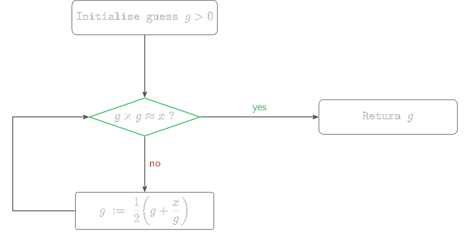
Consider Heron of Alexandria’s method for computing the square root of a real number, , such that is greater than 0.
- Initialise an arbitrary guess .
- If is sufficiently close to , terminate and return as the solution.
- Otherwise, assign a new value to the guess via the assignment operator introduced previously:
- Return to step 2.
This procedure illustrates the core architecture of computation: a sequence of operations governed by control flow. Control flow dictates execution order based on logical tests (which evaluate strictly to or ), allowing for the dynamic repetition or bypassing of instructions.
Problem 3
Let and initial guess . Using Heron’s method, compute the first three iterations of . Define “sufficiently close” as . Does the algorithm terminate within these three iterations?
Computability and Turing Completeness
Early computing machines were fixed-program computers, physically wired to solve exactly one specific mathematical problem. The advent of the stored-program computer fundamentally altered this paradigm. By storing both the sequence of instructions (the program) and the data it manipulates within the same memory space, a central interpreter can execute any legal set of instructions. A program counter directs the interpreter sequentially, deviating only when control flow dictates a jump. Because the result of a computation can itself be a new sequence of instructions, a modern computer is capable of programming itself.
To formalise the limits of what can be computed within this architecture, we rely on the theoretical model of the Universal Turing Machine (created in 1936 by Alan Turing).
The Church-Turing Thesis. If a mathematical function is computable, there exists a Turing Machine that can be programmed to compute it.
A programming language, such as Python, is termed Turing complete if it possesses the capacity to simulate a Universal Turing Machine. All standard modern programming languages share this property, rendering them fundamentally equivalent in raw computational power; all this means is that any algorithm expressible in one language can be theoretically expressed in another.
We noted previously that propositional logic is algorithmically decidable. General computation, however, loses this property. It is mathematically impossible to construct a universal algorithm that takes an arbitrary program as input and determines, in finite time, whether it will eventually halt or run indefinitely. This inherent limitation is known as the Halting Problem.
Syntax and Semantics
Just as mathematical logic is governed by syntax (the valid composition of symbols) and semantics (the truth value of that composition), All Programming languages strictly enforces these rules to eliminate ambiguity. When implementing algorithms, statements must pass three levels of structural verification:
- Primitive Constructs: The foundational building blocks of the language, including numeric literals (such as ), text strings, and operators (such as or ).
- Syntax: The grammatical rules dictating how primitives may be combined to form well-formed expressions. For example, the sequence is syntactically valid, whereas is not. Syntax errors are immediately caught by the interpreter prior to execution.
- Static Semantics: The rules determining whether a syntactically valid string possesses a logical meaning. For example, attempting to add a number to a text string may be syntactically structured correctly (Operand Operator Operand) but is statically invalid.
If a program is syntactically correct and free of static semantic errors, it possesses exact semantics. Unlike human language, every valid Python program has exactly one deterministic meaning.
If an algorithm behaves unexpectedly, it is not a failure of the language’s semantics, but a failure of the programmer’s logic. Such logical errors manifest in three ways: the program may crash during execution, it may enter an infinite loop, or (most dangerously) it may run to completion and produce an incorrect output. Consequently, rigorous mathematical verification of algorithms is required to ensure that logical deviations are self-evident.
Problem 4
For each of the following, state whether it results in a syntax error, a static semantic error, or produces unintended behavior (a logical error). Briefly justify.
x := 5 + * 3x := "hello" + 7- An implementation of Heron’s method that returns when instead of when is sufficiently small.
Instantiating Logic: Objects and Types
We now operationalise these concepts using Python. A Python program executes imperative knowledge via a sequence of definitions and commands, which are processed and evaluated sequentially by an interpreter.
A command, formally referred to as a statement, instructs the interpreter to perform a specific action. For instance, the print function outputs data to the execution environment. It accepts a variable number of arguments, which are by default separated by spaces when rendered. The output format can be controlled via keyword arguments, such as specifying end="" to suppress the default newline character.
# Sequential evaluation of commands
print("Algorithm")
print("terminated.")

# Supplying multiple arguments and controlling the end character
print("Algorithm", "terminated", end=".\n")
Computational Entities and Types
In mathematics, the validity of an operation depends entirely on the kind of entity it acts upon: addition is defined for numbers, conjunction for propositions, and so on. The computational analogue of such an entity is an object. Every object in Python possesses a specific type, which definitively dictates the operations legally permitted upon that object.
This strict typing system is the mechanism by which the interpreter enforces the static semantics discussed previously. Types bifurcate into two fundamental categories: scalar and non-scalar. Scalar objects are structurally indivisible, acting as the atomic elements of the language, whereas non-scalar objects (such as text strings) possess internal structure.
Python implements four primitive scalar types:
int: Represents the integers. Literals are denoted standardly (e.g.,5,-12).float: Approximates the real numbers. Literals must include a decimal point (e.g.,3.0,-28.72) or use scientific notation. Because computational memory is finite, continuous reals are represented using discrete floating-point structures. This architectural necessity introduces slight deviations from pure real arithmetic, a fundamental limitation of discrete computation that we will address later.bool: The executable manifestation of the truth values established in Definition 2. It is inhabited by exactly two values:True(corresponding to ) andFalse(corresponding to ).None: A type inhabited by a singular null value, used to define an empty state or the absence of a returned object.
Expressions and Relational Operators
When objects and operators are validly combined according to the language’s syntax, they form an expression. Just as a mathematical term can be simplified, an expression inherently evaluates to a singular object of a defined type. The built-in function type() permits the dynamic inspection of an object’s classification.
type(5) # Evaluates to: int

type(5.0) # Evaluates to: float
The construction of algorithms relies heavily on control flow, which in turn requires evaluating atomic propositions (Definition 3) to strictly or . We achieve this computationally using relational operators.
Crucially, the syntax for assignment and logical equivalence diverge. In our earlier mathematical notation, we distinguished assignment () from equality (). Python syntax maps mathematical assignment to the single equals sign =. To test whether two expressions evaluate to identical values, we must use the logical equivalence operator ==, while non-equivalence is denoted by !=.
The evaluation of a relational operator always yields a bool. Thus, an expression such as 3 != 2 is a fully formed atomic proposition within the machine’s logic.
# Evaluating an arithmetic expression
3.0 + 2.0 # Evaluates to the float: 5.0

# Evaluating a relational proposition
3 != 2 # Evaluates to the bool: True
Problem 5
Consider the Python expressions type(4 == 4) and type(4.0). Determine the output of both. Explain how the distinction between = and == prevents static semantic errors when constructing the logical tests required for the control flow of algorithms, such as step 2 of Heron’s method.
Arithmetic Operators and Precedence
Computation requires the precise articulation of operations upon objects. The arithmetic operators applicable to int and float types closely mirror standard mathematical notation, yet they introduce critical distinctions necessitated by the discrete nature of machine architecture.
The standard arithmetic operators include addition (+), subtraction (-), and multiplication (*). Exponentiation is denoted by **.
A fundamental structural divergence from pure mathematics arises with division. Python implements two distinct division operators:
- Standard Division (
/): Invariably evaluates to afloat, providing an approximation of division within . For instance,5 / 3evaluates to1.6666666666666667. - Floor Division (
//): Performs integer division, discarding the fractional remainder to return the largest integer less than or equal to the quotient. Thus,5 // 3evaluates to1, and-4 // 3evaluates to-2. - Modulo (
%): Evaluates to the remainder of the integer division. For example,5 % 3evaluates to2. The modulo operator is foundational to discrete mathematics and will form the computational basis for our later exploration of modular arithmetic and Number Theory.
Problem 6
Verify that (a%b) is equivalent to (a - (a//b)*b).
When constructing compound expressions, the interpreter strictly adheres to an order of operator precedence. Exponentiation (**) binds most tightly, followed by multiplication and division operators (*, /, //, %), and finally addition and subtraction (+, -).
print(2 + 3 * 4)  # prints 14, not 20
print(5 + 4 % 3)  # prints  6, not 0 (% has same precedence as *, /, and //)
print(2 ** 3 * 4) # prints 32, not 4096 (** has higher precedence than *, /, //, and %)
Furthermore, operations of equal precedence are governed by associativity. While most operators associate strictly left-to-right, exponentiation associates right-to-left.
print(5-4-3)   # prints -2, not 4 (- associates left-to-right)

# Right-to-left associativity of exponentiation
4 ** 3 ** 2 # Evaluates to 4 ** 9 (262144), not 64 ** 2 (4096)

# Parentheses rigorously dictate evaluation order
(4 ** 3) ** 2 # Evaluates to 4096
Propositional Logic in Computation
The logical connectives established in our formal syntax—negation (), conjunction (), and disjunction ()—are implemented natively in Python via the reserved keywords not, and, and or. These primitive operators act strictly upon objects of type bool and strictly enforce the truth tables defined previously.
Because they are reserved keywords, they are an intrinsic part of the language’s syntax and cannot be redefined or used as variable names. This guarantees that logical tests within algorithms remain deterministic and free from semantic ambiguity.
# Evaluates a formal conjunction
(3 != 2) and (5 % 3 == 0) # Evaluates to: False (since 5 % 3 == 2, the second proposition is False)
Python Operator Summary
| Category | Operators |
|---|---|
| Arithmetic | +, -, *, /, //, **, %, unary -, unary + |
| Relational | <, <=, >=, >, ==, != |
| Assignment | +=, -=, *=, /=, //=, **=, %=, <<=, >>= |
| Logical | and, or, not |
For now, we are not covering the bitwise operators (<<, >>, &, |, ^, ~, &=, |=, ^=). Since <<= and >>= depend on bitwise shifts, we will also defer using them in this lesson.
Variable Binding and State
In mathematics, an equation such as establishes a permanent, structural equivalence between the left and right sides. If varies, intrinsically varies with it.
In imperative programming, this is emphatically not the case. The assignment statement = dictates a temporal binding. A variable in Python is simply a human-readable identifier bound to a specific computational object in memory.
Consider the following sequence of instructions calculating the area of a circle:
pi = 3.14159
radius = 11.0
area = pi * (radius ** 2)
radius = 14.0
The third statement evaluates the expression pi * (radius ** 2) down to a singular float object (379.94039), and binds the identifier area to that object. When the fourth statement re-binds radius to 14.0, it has absolutely no effect on the value to which area is bound. The state of area remains fixed until it is explicitly reassigned.
This strict separation of temporal states is what allows algorithms, such as Heron’s method, to iteratively update a guess () without destroying the fundamental properties of the initial input ().
Code Semantics and Readability
Because programs dictate complex logical flow, their mathematical correctness must be verifiable by human readers. A syntactically valid program can still be semantically nonsensical if its identifiers obscure its logic. Naming identifiers clearly and using the # symbol to append non-executable comments are vital practices for maintaining mathematical clarity.
# Correct mathematical semantics but poor variable naming
a = 3.14159
b = 11.2
c = a * (b ** 2)

# Identical execution, but logically verifiable
pi = 3.14159
diameter = 11.2
area = pi * ((diameter / 2.0) ** 2)
By reading the second block, a mathematician immediately identifies a logical error in the first block (failing to halve the diameter before squaring it).
Multiple Assignment
Python provides a mechanism for binding multiple variables simultaneously. The assignment sequence evaluates every expression on the right-hand side of the = operator completely before altering any of the bindings on the left-hand side.
This atomic evaluation enables elegant manipulations of algorithmic state, such as swapping the values of two variables without requiring an intermediate, temporary variable:
x, y = 2, 3

# The expressions on the right are evaluated to objects (3, 2)
# before the names x and y are rebound.
x, y = y, x

print("x is", x) # Outputs: x is 3
print("y is", y) # Outputs: y is 2
Problem 7
Consider the multiple assignment a, b = 1, 1 followed by the iterative step a, b = b, a + b. If this step is executed three times in succession, what are the final bound values of a and b? Relate this sequence to a well-known mathematical sequence.
The Structure of Proof Systems
We have established a language of propositions, connectives, and truth tables. We have also built a computational toolkit capable of evaluating these constructs mechanically. The natural question is: what can we actually do with all of this?
Truth tables answer individual questions. Given a compound proposition, we can enumerate every possible assignment and read off the result. But this brute enumeration scales poorly. A formula with atomic variables demands rows. More fundamentally, a truth table tells us that something is true without revealing why it is true, or how its truth connects to anything else. Mathematics demands more than verification; it demands structure.
A proof system provides exactly this structure. It consists of two classes of objects: statements (finite strings of symbols expressing propositions) and proofs (finite strings of symbols justifying those statements). The relationship between them is governed by two functions:
- Semantics (Truth): A rule determining whether a given statement is true or false. In our previous work, truth tables served this role.
- Verification (Syntax): A mechanical procedure that decides whether a specific string constitutes a valid proof for a given statement. This verification must be efficiently computable; a proof whose validity cannot be checked in reasonable time is operationally useless.
These two functions give rise to two critical properties. A proof system is sound if no false statement possesses a valid proof: the verification procedure never accepts a justification for an untruth. A proof system is complete if every true statement possesses a valid proof: nothing true escapes the reach of the system.
Consider statements of the form “The integer is composite.”
- Semantics: The statement is true if has a divisor such that .
- Proof: A valid proof could simply be the divisor itself.
- Verification: Divide by and check whether the remainder is zero.
The verification step is computationally cheap, even when finding the divisor is extraordinarily difficult. This asymmetry between the difficulty of discovery and the ease of verification is a recurring theme in both mathematics and computer science.
# Verification of compositeness: given n and a candidate divisor d
n = 91
d = 7
# The verification is a single arithmetic check
n % d == 0 and 1 < d < n # Evaluates to: True (91 = 7 * 13, so 91 is composite)
We now build a proof system for propositional logic itself.
Satisfiability
Before constructing proofs, we must classify propositions by the range of truth values they can assume. Not all compound propositions behave alike: some are always true, some are always false, and some depend on the assignment.
A compound proposition is a tautology if it evaluates to under every possible assignment of truth values to its atomic variables.
A compound proposition is a contradiction if it evaluates to under every possible assignment of truth values to its atomic variables.
A compound proposition is a contingency if it is neither a tautology nor a contradiction; its truth value depends on the specific assignment.
A proposition is satisfiable if there exists at least one assignment under which it evaluates to . Every tautology and every contingency is satisfiable. A contradiction is unsatisfiable.
The proposition is a tautology (by the Principle of Bivalence, one of or must hold). The proposition is a contradiction. The bare variable is a contingency.
To establish that a proposition is satisfiable, a single witness assignment suffices. To establish that it is unsatisfiable, one must check every assignment, which is precisely the expensive enumeration that motivates the algebraic approach developed below.
# Witness for satisfiability: one assignment suffices
# Is (p or not q) and (q or not r) and (r or not p) satisfiable?
p, q, r = True, True, True
(p or not q) and (q or not r) and (r or not p) # Evaluates to: True — one witness is enough
Problem 8
Determine the satisfiability of . If satisfiable, provide a witness assignment. If unsatisfiable, justify your answer.
Axioms and Equivalence Proofs
We now introduce the axiomatic foundation that allows us to reason about propositional equivalences without enumerating truth tables. The axioms of classical propositional logic specify the algebraic behaviour of the connectives , , and . Each axiom is a logical equivalence, asserting that two expressions are interchangeable in all contexts. The first five axiom pairs define a structure known as a Boolean algebra.
Two additional axioms disintegrate the conditional connectives into the core trio :
The Conditional axiom deserves special attention. It asserts that every implication can be rewritten using only negation and disjunction. This means the implication symbol is, strictly speaking, syntactic convenience rather than a primitive operation. Its presence in the “antecedent position” introduces a hidden negation, which is the source of much confusion when manipulating implications algebraically.
From these axioms, we derive theorems. Recall Definition 4: a proof begins from known truths and proceeds via valid logical steps. An equivalence proof is a chain of equivalences, each justified by an axiom, a definition, or a previously established theorem:
This method is vastly more efficient than truth tables for complex formulas, though it requires algebraic ingenuity rather than mechanical enumeration.
Fundamental Theorems
For any propositions and , if and , then .
Let and be arbitrary propositions satisfying and . We show that both and reduce to the same expression. First:
Similarly:
Both and equal , hence .
■This theorem is the engine behind nearly every derivation that follows. It tells us that if something behaves like a complement (annihilates under , completes under ), then it is the complement. We now put it to work.
and .
By Identity, . By Commutativity and Identity, . The premises of Theorem 1 are satisfied with and , yielding . The second statement follows identically with , .
■For any propositions and , if , then .
Let . Then:
By Theorem 1 (with playing the role of and playing the role of ), we conclude .
■For any propositions such that and :
The proofs are straightforward applications of substitution and are omitted.
With Theorem 1 and its corollaries established, we can now derive the classical theorems of propositional logic.
For any proposition , .
By Complement (and Commutativity): and . The premises of Theorem 1 are met with in the role of and in the role of . Therefore .
■# Double Negation: quick computational check
p = True
p == (not (not p)) # Evaluates to: True
p = False
p == (not (not p)) # Evaluates to: TrueFor any proposition , and .
For the conjunctive case:
The disjunctive case follows analogously:
■For any proposition , and .
For the disjunctive fragment:
The conjunctive fragment:
■For any propositions and , and .
For the disjunctive case:
The conjunctive case:
■For any propositions and , and .
We prove by applying Theorem 1. We must show and .
The conjunctive branch:
The disjunctive branch:
By Theorem 1, . The proof of is analogous.
■# De Morgan's Laws: computational verification
p, q = True, False
not (p and q) == (not p or not q) # Evaluates to: True
p, q = False, True
not (p or q) == (not p and not q) # Evaluates to: TrueThe symbol at the end of a proof is a modern substitute for the traditional Q.E.D., an initialism for the Latin phrase quod erat demonstrandum, meaning “what was to be shown.”
Problem 9
Prove by equivalence proof that (the second De Morgan’s Law). Hint. Apply Theorem 1 as in the proof of Theorem 6.
Equivalences Involving Conditionals
The Conditional axiom () and the Biconditional axiom allow us to derive every conditional equivalence by reducing implications to and applying the theorems above:
Notice the pattern in the implication equivalences: when implications share the same premise, the conclusions combine with the same connective ( or ). When they share the same conclusion, the premises combine with the opposite connective. This “flip” from to (and vice versa) is a direct consequence of the hidden negation in the Conditional axiom: the antecedent of an implication sits behind a , so De Morgan’s Laws invert the connective when premises are merged.
Contrapositive, Converse, and Inverse
From an implication , three related conditionals arise:
- The contrapositive is logically equivalent to . This equivalence () is one of the most powerful proof techniques in mathematics.
- The converse is not equivalent to . We proved this nonequivalence in Definition 6 via a counterexample.
- The inverse is the contrapositive of the converse, hence equivalent to but not to .
The converse and inverse are equivalent to each other. Confusing an implication with its converse is a pervasive logical fallacy.
Equivalence Proofs in Practice
We now work through several examples that demonstrate the method and, simultaneously, show how Python can serve as a rapid sanity check.
Show that .
# Quick validation across all assignments
p, q = True, True
not (p or (not p and q)) == (not p and not q) # Evaluates to: True

p, q = False, True
not (p or (not p and q)) == (not p and not q) # Evaluates to: TrueShow that is a tautology.
The formula reduces to with no surviving variables, confirming it is a tautology regardless of assignment.
Show that .
This result captures a natural proof strategy: to show that a disjunction implies something, it suffices to show that each disjunct separately implies it.
The negation of “If I think, then I am” () is:
by the Conditional axiom and De Morgan (Theorem 6). So the negation is “I think and I am not.” Negating an implication does not produce another implication; it produces a conjunction where the premise holds and the conclusion fails.
This is the only scenario under which an implication is false, consistent with the truth table established earlier.
# The only way an implication fails
p, q = True, False
(p and not q) == (not (not p or q)) # Evaluates to: TrueIs distributive over and ?
The claim holds. Expanding both sides via the definition :
Left side:
Right side:
Both sides reduce to the same expression. However, fails.
A single counterexample suffices: set , , .
# Counterexample for disjunctive distributivity of XOR
p, q, r = True, True, True
lhs = p or (q != r)  # XOR via != on bools
rhs = (p or q) != (p or r)
lhs == rhs # Evaluates to: False — the equivalence fails
Problem 10
Using equivalence proofs (not truth tables), show that . This establishes the contrapositive equivalence from first principles.
Problem 11
Show, using an equivalence proof, that . Identify precisely where the “flip” from to the structure of the result occurs, and which axiom is responsible.
Problem 12
The negation of “Candidates must have a degree in mathematics or computer science” is not “Candidates must have a degree in mathematics and computer science.” Using the propositions = “The candidate has a degree in mathematics” and = “The candidate has a degree in computer science”, express the original statement formally as an implication and compute its negation. Identify the De Morgan’s Law involved.
Normal Forms
We Finish off this session with Normal forms.
The equivalence proofs developed above demonstrate that any compound proposition can be transformed into an equivalent expression using only the core connectives , , and . But this raises a question: given two arbitrary propositions, how do we determine whether they are equivalent without the algebraic ingenuity required for an equivalence proof? Truth tables answer this mechanically, but they scale exponentially.
A normal form solves this by being a fixed structural template for propositional formulas. If two propositions are equivalent, their normal forms will be identical (after simplification). This converts the semantic question “do these formulas always agree?” into the syntactic question “do these strings match?” The practical consequences extend well beyond theorem-proving. Normal forms underpin circuit design (where logical gates physically instantiate , , ), automated verification systems, and, as we shall see, some of the open questions in computational complexity.
Before defining the two principal normal forms, we need precise terminology for their building blocks.
A literal is a propositional variable or its negation. If is a propositional variable, then both and are literals.
A clause is a disjunction or conjunction of literals. A disjunctive clause (or simply a clause in the context of CNF) is a disjunction of literals. A conjunctive clause (or term) is a conjunction of literals.
Disjunctive Normal Form
A propositional formula is in Disjunctive Normal Form (DNF) if it consists of a disjunction of one or more terms, where each term is a conjunction of literals. That is, DNF has the shape:
where each is a literal.
The structure is: OR of ANDs. Each conjunctive term describes one specific scenario under which the formula holds; the overall disjunction asserts that at least one of these scenarios is realised.
The following formulas are in DNF:
- . Two terms, each a conjunction of two literals.
- . A single literal is a degenerate term (a conjunction of one literal).
- .
The following formulas are not in DNF:
- . The negation is not a literal; it is a negated compound expression that must first be expanded via De Morgan’s Laws (Theorem 6).
- . This is a conjunction of a disjunctive clause with a term: the outer connective is , not .
- . A negated disjunction, not a disjunction of conjunctions.
Constructing DNF from Truth Tables
Every compound proposition can be mechanically converted to DNF via its truth table. The procedure is:
- Construct the truth table for the proposition.
- Identify every row where the proposition evaluates to .
- For each such row, form a conjunctive term: include the variable if it is assigned in that row, or if it is assigned .
- Take the disjunction of all such terms.
The resulting formula is in DNF by construction. Each term encodes exactly one satisfying assignment, and the disjunction collects them all.
Find the DNF of .
We construct the truth table:
Rows 2, 4, 6, 7, 8 evaluate to . Reading off each row:
This is the full DNF. It can be simplified using the equivalence (which follows from Distributivity and Complement). Group the first two terms:
For the last three terms, observe that we may use Idempotence (Theorem 3) to duplicate the fifth term () without altering the formula. This allows two independent groupings:
Combining:
Applying the Conditional axiom and De Morgan (Theorem 6) in reverse: . The simplified DNF recovers the original formula, confirming equivalence.
# Verify DNF equivalence
p, q, r = True, True, True
original = (not (p or q)) or (not r)
dnf = (p and q and not r) or (p and not q and not r) or (not p and q and not r) or (not p and not q and r) or (not p and not q and not r)
simplified = (not r) or (not p and not q)
print(original == dnf == simplified) # True

p, q, r = True, True, False
original = (not (p or q)) or (not r)
dnf = (p and q and not r) or (p and not q and not r) or (not p and q and not r) or (not p and not q and r) or (not p and not q and not r)
simplified = (not r) or (not p and not q)
print(original == dnf == simplified) # True

# ... and so on for all 8 assignments
Conjunctive Normal Form
A propositional formula is in Conjunctive Normal Form (CNF) if it consists of a conjunction of one or more clauses, where each clause is a disjunction of literals. That is, CNF has the shape:
where each is a literal.
The structure is: AND of ORs, the dual of DNF. Each disjunctive clause represents a constraint that must be satisfied; the conjunction demands that every constraint holds simultaneously.
The following formulas are in CNF:
- .
- .
The following formulas are not in CNF:
- . The outer connective is , and the operands are conjunctions, not disjunctions. This is DNF, not CNF.
- . A negated disjunction, not a conjunction of disjunctive clauses.
Constructing CNF
There are two systematic methods for obtaining CNF.
Method 1: Algebraic manipulation. Eliminate all implications using the Conditional and Biconditional axioms. Push negations inward using De Morgan’s Laws (Theorem 6) and Double Negation (Theorem 2). Then distribute over using the equivalence (the disjunctive form of Distributivity) until every clause is a disjunction of literals.
Method 2: Truth table (via negation of DNF). Observe that by Double Negation (Theorem 2), any proposition satisfies . Construct the DNF of by reading off the rows where evaluates to (equivalently, where evaluates to ). Then negate the resulting DNF. By De Morgan’s Laws (Theorem 6), negating a disjunction of conjunctions produces a conjunction of disjunctions: precisely CNF.
Find the CNF of .
Method 1 (Algebraic):
Method 2 (Truth table):
The formula evaluates to in rows 5 and 7. Form the DNF of the negation by reading these rows:
Simplify: . Now negate:
by De Morgan (Theorem 6) and Double Negation (Theorem 2). This is already in CNF.
Method 2 produced , while Method 1 produced . These are equivalent: the second clause in Method 1’s result is absorbed by the first via Absorption (Theorem 5), since any assignment satisfying automatically satisfies .
# Verify both CNF forms match the original
p, q, r = False, True, True
original = (not (not p or q)) or (not r or p)
cnf1 = (p or not r) and (p or not q or not r)
cnf2 = p or not r
print(original == cnf1 == cnf2) # True

p, q, r = False, False, True
original = (not (not p or q)) or (not r or p)
cnf1 = (p or not r) and (p or not q or not r)
cnf2 = p or not r
print(original == cnf1 == cnf2) # True
The Cost of Canonicality
Normal forms guarantee a canonical structure, but this guarantee comes at a price. Converting between normal forms can cause an exponential blowup in the number of clauses.
Consider a formula already in DNF with terms:
To convert this to CNF, we must distribute over repeatedly. Each application of Distributivity doubles the number of clauses. Starting with :
Two terms in DNF produce four clauses in CNF. Adjoining a third term via disjunction and distributing again doubles to eight clauses. After terms, the CNF may contain up to clauses. The symmetric explosion occurs when converting CNF to DNF.
This exponential blowup is an intrinsic property of the normal forms themselves. It is also the reason why the satisfiability of CNF formulas (the SAT problem) occupies a central position in complexity theory: determining whether a CNF formula has a satisfying assignment is the canonical NP-complete problem, meaning that no known algorithm solves it efficiently in all cases.
Problem 13
Find the DNF of using the truth table method. Simplify the result.
Problem 14
Convert into DNF using algebraic manipulation (Distributivity, not truth tables). Verify your result computationally.
Problem 15
Find the CNF of using both methods (algebraic and truth table). Confirm that both methods yield equivalent results.
Application: Knights and Knaves
Normal forms and propositional reasoning converge naturally in logic puzzles, where the challenge is to deduce facts from constrained declarations. Consider the following scenario.
On an island, every inhabitant is either a knight (who always tells the truth) or a knave (who always lies). You encounter two inhabitants, and .
- says: “B is a knight.”
- says: “The two of us are of opposite types.”
Let denote ” is a knight” and denote ” is a knight.” We translate the scenario into propositional logic.
If is a knight ( is ), then ‘s statement is true, so is . If is a knave ( is ), then ‘s statement is false, so is . In both cases, ‘s declaration encodes .
’s statement asserts that and are of opposite types, which means exactly one of is : this is . If is a knight ( is ), then must be . If is a knave ( is ), then must be . So ‘s declaration encodes .
The full constraint is:
Case 1: Assume is . From , we get is . Then . But . The conjunction evaluates to . Contradiction.
Case 2: Assume is . From , we get is . Then . And . The conjunction evaluates to .
Therefore both and are knaves.
# Test all four assignments of (p, q)
p, q = True, True
print((p == q) and (q == (p != q))) # False

p, q = True, False
print((p == q) and (q == (p != q))) # False

p, q = False, True
print((p == q) and (q == (p != q))) # False

p, q = False, False
print((p == q) and (q == (p != q))) # True — both knaves
Problem 16
On the same island, you meet three inhabitants , , and . says: “All of us are knaves.” says: “Exactly one of us is a knight.” Using propositional variables , , for , , respectively, determine the types of all three inhabitants. Verify your solution computationally.