03/03/2026

#Math#Vectors#Geometry

Video

Lesson assets

video link

CS50P Lecture 0: Functions, Variables

recitation

Recitation 1 PDF

Homework 1 PDF

Vectors and Plane Geometry

We have now developed sufficient algebraic machinery to revisit plane geometry through the lens of vectors. Rather than reformulating the entirety of Euclidean geometry, we establish a dictionary between the geometric properties of the plane and the algebraic structure of the vector space $\mathbb{R}^2$ . This correspondence allows us to prove geometric theorems with algebraic rigour.

Position and Displacement Vectors

Definition 10 (Position Vector)

Let $O = (0,0)$ be the origin of the Cartesian plane. For any point $A = (a_1, a_2)$ , the vector $\mathbf{a} = \begin{bmatrix} a_1 \\ a_2 \end{bmatrix}$ represented by the directed segment $\overrightarrow{OA}$ is called the position vector of $A$ .

Through this convention, every point in the plane is uniquely associated with a vector. The position vector of a point is simply the vector whose components are the coordinates of that point. While position vectors are “bound” to the origin, we also need vectors between arbitrary points.

Definition 11 (Displacement Vector)

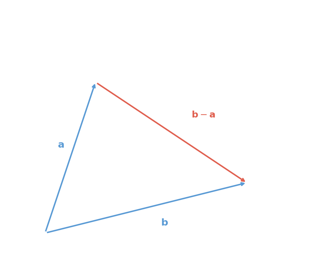
Let $A$ and $B$ be distinct points with position vectors $\mathbf{a}$ and $\mathbf{b}$ respectively. The directed segment $\overrightarrow{AB}$ is represented by the vector

\overrightarrow{AB} = \mathbf{b} - \mathbf{a}.

This vector is called the displacement vector from $A$ to $B$ .

Remark

This definition is consistent with the triangle rule for vector addition. The chain $\overrightarrow{OA} + \overrightarrow{AB} = \overrightarrow{OB}$ implies $\mathbf{a} + \overrightarrow{AB} = \mathbf{b}$ , so $\overrightarrow{AB} = \mathbf{b} - \mathbf{a}$ . Observe that reversing direction negates the vector: $\overrightarrow{BA} = \mathbf{a} - \mathbf{b} = -\overrightarrow{AB}$ .

Position vectors a and b from the origin to points A and B, and the displacement vector b minus a from A to B

With position and displacement vectors in hand, fundamental geometric properties translate directly into vector notation.

Distance: The length of the segment $AB$ is the magnitude of the displacement vector: $d(A,B) = |\mathbf{b} - \mathbf{a}|$ .
Collinearity: Three distinct points $A, B, C$ are collinear if and only if the displacement vectors $\overrightarrow{AB}$ and $\overrightarrow{AC}$ are linearly dependent (Definition 9). That is, $\mathbf{b}-\mathbf{a} = k(\mathbf{c}-\mathbf{a})$ for some scalar $k$ .
Parallelograms: A quadrilateral $ABCD$ is a parallelogram if and only if $\overrightarrow{AB} = \overrightarrow{DC}$ , which in terms of position vectors reads $\mathbf{b} - \mathbf{a} = \mathbf{c} - \mathbf{d}$ .

Example 7

Let $A = (1, 3)$ , $B = (4, 1)$ , and $C = (7, -1)$ . The displacement vectors are:

\overrightarrow{AB} = \begin{bmatrix} 3 \\ -2 \end{bmatrix}, \qquad \overrightarrow{AC} = \begin{bmatrix} 6 \\ -4 \end{bmatrix} = 2\begin{bmatrix} 3 \\ -2 \end{bmatrix} = 2\,\overrightarrow{AB}.

Since $\overrightarrow{AC}$ is a scalar multiple of $\overrightarrow{AB}$ , the three points are collinear. The distance from $A$ to $B$ is $|\overrightarrow{AB}| = \sqrt{9 + 4} = \sqrt{13}$ .

Example 8

Let $P = (2, 1)$ , $Q = (5, 3)$ , and $R = (3, 4)$ . Are these three points collinear?

\overrightarrow{PQ} = \begin{bmatrix} 3 \\ 2 \end{bmatrix}, \qquad \overrightarrow{PR} = \begin{bmatrix} 1 \\ 3 \end{bmatrix}.

If $\overrightarrow{PR} = k\,\overrightarrow{PQ}$ , then $1 = 3k$ and $3 = 2k$ , giving $k = 1/3$ and $k = 3/2$ respectively. These are inconsistent, so no such $k$ exists. Alternatively, the determinant (Theorem 5) is $3 \cdot 3 - 2 \cdot 1 = 7 \neq 0$ . The three points are not collinear; they form a triangle.

The Midpoint Formula

Theorem 9 (Midpoint Formula)

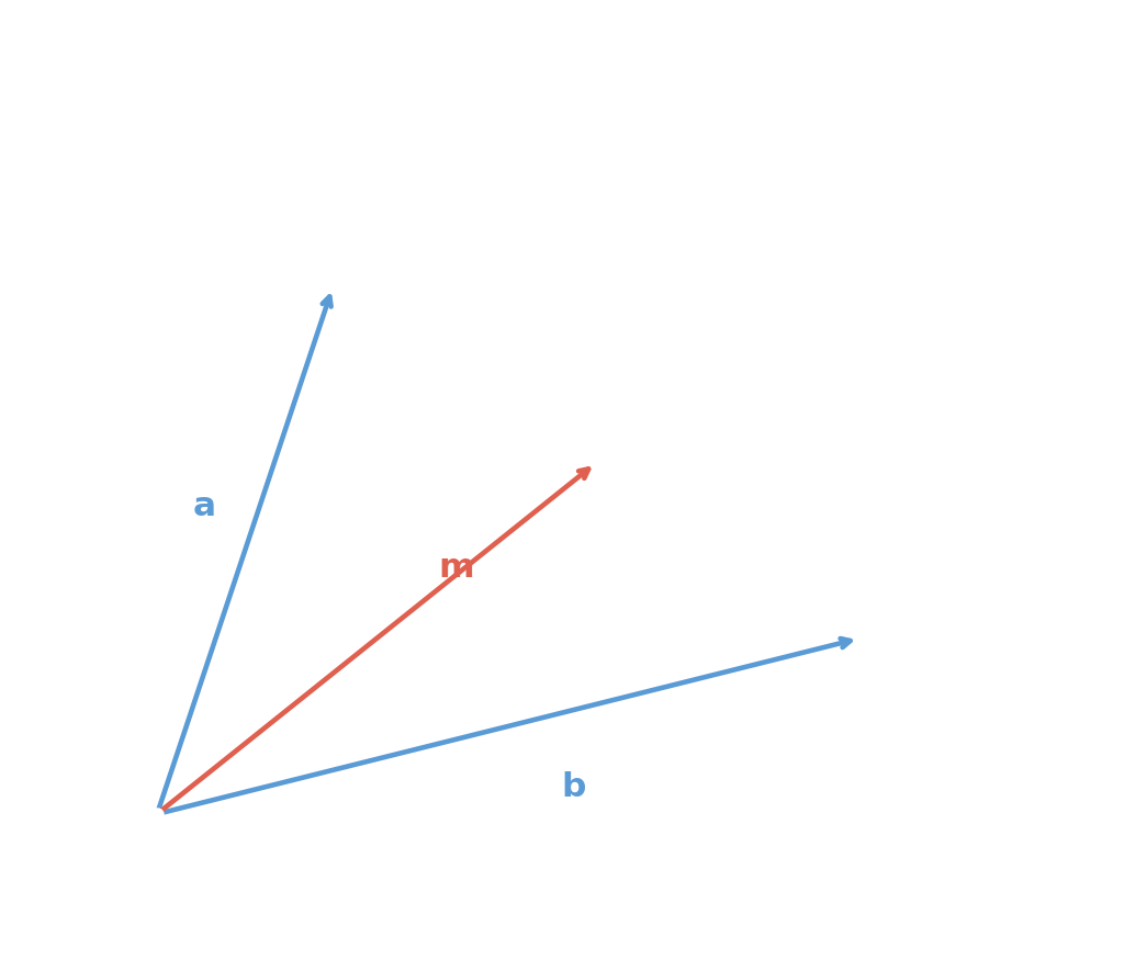
Let $A$ and $B$ be points with position vectors $\mathbf{a}$ and $\mathbf{b}$ . The midpoint $M$ of the segment $\overline{AB}$ has the position vector

\mathbf{m} = \frac{1}{2}(\mathbf{a} + \mathbf{b}).

Proof

Let $M$ be the midpoint of $\overline{AB}$ . By definition, $M$ divides the segment into two equal parts, so the displacement from $A$ to $M$ equals the displacement from $M$ to $B$ :

\overrightarrow{AM} = \overrightarrow{MB}.

In terms of position vectors, $\mathbf{m} - \mathbf{a} = \mathbf{b} - \mathbf{m}$ . Adding $\mathbf{m}$ to both sides gives $2\mathbf{m} = \mathbf{a} + \mathbf{b}$ , whence $\mathbf{m} = \frac{1}{2}(\mathbf{a} + \mathbf{b})$ .

■

The midpoint is therefore the average of the two position vectors.

The position vector of the midpoint M is the average of a and b

Example 9

For $A = (1, 3)$ and $B = (4, 1)$ , the midpoint is

M = \frac{1}{2}\left(\begin{bmatrix} 1 \\ 3 \end{bmatrix} + \begin{bmatrix} 4 \\ 1 \end{bmatrix}\right) = \frac{1}{2}\begin{bmatrix} 5 \\ 4 \end{bmatrix} = \left(\frac{5}{2},\; 2\right).

Problem 6

Let $A = (3, -1)$ and $M = (5, 2)$ , where $M$ is the midpoint of $\overline{AB}$ . Determine the coordinates of $B$ .

Parallelogram Diagonals

Using the midpoint formula, we can prove a classical result about parallelograms with almost no computation.

Theorem 10 (Parallelogram Diagonals)

The diagonals of a parallelogram bisect each other.

Proof

Let $ABCD$ be a parallelogram with position vectors $\mathbf{a}, \mathbf{b}, \mathbf{c}, \mathbf{d}$ . Since $ABCD$ is a parallelogram, opposite sides are equal and parallel: $\overrightarrow{AB} = \overrightarrow{DC}$ . In terms of position vectors, $\mathbf{b} - \mathbf{a} = \mathbf{c} - \mathbf{d}$ , which rearranges to

\mathbf{a} + \mathbf{c} = \mathbf{b} + \mathbf{d}.

The midpoint of diagonal $AC$ has position vector $\mathbf{m}_1 = \frac{1}{2}(\mathbf{a} + \mathbf{c})$ , and the midpoint of diagonal $BD$ has position vector $\mathbf{m}_2 = \frac{1}{2}(\mathbf{b} + \mathbf{d})$ . Since $\mathbf{a} + \mathbf{c} = \mathbf{b} + \mathbf{d}$ , it follows that $\mathbf{m}_1 = \mathbf{m}_2$ . The midpoints of the diagonals coincide, so the diagonals bisect each other.

■

Example 10

Let $A = (0,0)$ , $B = (3,1)$ , $D = (1,2)$ . For $ABCD$ to be a parallelogram, we need $\overrightarrow{AB} = \overrightarrow{DC}$ , so $C = B + D - A = (4, 3)$ . The midpoint of $AC$ is $\frac{1}{2}(0+4,\;0+3) = (2,\; 3/2)$ . The midpoint of $BD$ is $\frac{1}{2}(3+1,\;1+2) = (2,\; 3/2)$ . The diagonals bisect each other, as the theorem guarantees.

Problem 7

A quadrilateral $ABCD$ has vertices $A = (1, 0)$ , $B = (4, 1)$ , $C = (5, 4)$ , $D = (2, 3)$ . Verify that $ABCD$ is a parallelogram by checking $\overrightarrow{AB} = \overrightarrow{DC}$ . Then confirm that the midpoints of the diagonals coincide.

The Parametric Equation of a Line

We established above that a point $X$ lies on the line passing through $A$ and $B$ if and only if the vectors $\overrightarrow{AX}$ and $\overrightarrow{AB}$ are linearly dependent. The parametric equation makes this condition explicit by expressing every point on the line in terms of a single real parameter.

Theorem 11 (Parametric Line Equation)

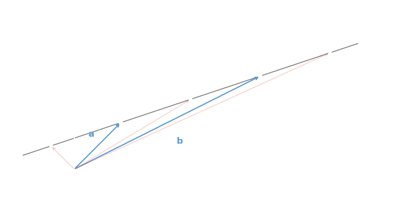
Let $A$ and $B$ be distinct points with position vectors $\mathbf{a}$ and $\mathbf{b}$ . A point $X$ lies on the line $L_{AB}$ if and only if its position vector $\mathbf{x}$ satisfies

\mathbf{x} = (1-t)\,\mathbf{a} + t\,\mathbf{b}

for some scalar $t \in \mathbb{R}$ .

Proof

Suppose $X$ lies on $L_{AB}$ . Then $\overrightarrow{AX}$ is parallel to $\overrightarrow{AB}$ , so $\overrightarrow{AX} = t\,\overrightarrow{AB}$ for some scalar $t$ . In terms of position vectors:

\mathbf{x} - \mathbf{a} = t(\mathbf{b} - \mathbf{a}).

Rearranging: $\mathbf{x} = \mathbf{a} + t\mathbf{b} - t\mathbf{a} = (1-t)\mathbf{a} + t\mathbf{b}$ .

Conversely, if $\mathbf{x} = (1-t)\mathbf{a} + t\mathbf{b}$ , then $\mathbf{x} - \mathbf{a} = t(\mathbf{b} - \mathbf{a})$ , so $\overrightarrow{AX} = t\,\overrightarrow{AB}$ , which means $\overrightarrow{AX}$ and $\overrightarrow{AB}$ are linearly dependent and $X$ lies on $L_{AB}$ .

■

The scalar $t$ is the parameter. The position of $X$ relative to $A$ and $B$ is determined entirely by $t$ :

$t = 0$ gives $\mathbf{x} = \mathbf{a}$ , so $X = A$ .
$t = 1$ gives $\mathbf{x} = \mathbf{b}$ , so $X = B$ .
$0 < t < 1$ places $X$ strictly between $A$ and $B$ , on the segment $\overline{AB}$ .
$t > 1$ places $X$ beyond $B$ , so that $B$ lies between $A$ and $X$ .
$t < 0$ places $X$ beyond $A$ in the opposite direction, so that $A$ lies between $X$ and $B$ .

Points on the line through A and B determined by the parameter t

Remark

The midpoint formula (Theorem 9) is a special case of the parametric line equation with $t = 1/2$ :

\mathbf{x} = \tfrac{1}{2}\mathbf{a} + \tfrac{1}{2}\mathbf{b} = \tfrac{1}{2}(\mathbf{a} + \mathbf{b}).

Example 11

Let $A = (1, 2)$ and $B = (4, 5)$ . The point on $L_{AB}$ with parameter $t = 2/3$ is

\mathbf{x} = \frac{1}{3}\begin{bmatrix} 1 \\ 2 \end{bmatrix} + \frac{2}{3}\begin{bmatrix} 4 \\ 5 \end{bmatrix} = \begin{bmatrix} 1/3 + 8/3 \\ 2/3 + 10/3 \end{bmatrix} = \begin{bmatrix} 3 \\ 4 \end{bmatrix}.

Since $0 < 2/3 < 1$ , this point lies on the segment $\overline{AB}$ , two-thirds of the way from $A$ to $B$ .

Problem 8

Let $A = (2, -1)$ and $B = (6, 7)$ . Find the parameter $t$ such that the point $X$ on $L_{AB}$ has coordinates $(5, 5)$ . Verify that this value of $t$ lies in the interval $(0, 1)$ , confirming that $X$ is between $A$ and $B$ .

Concurrency and the Centroid

The parametric representation is particularly powerful for proving concurrency theorems: results asserting that several lines pass through a single common point.

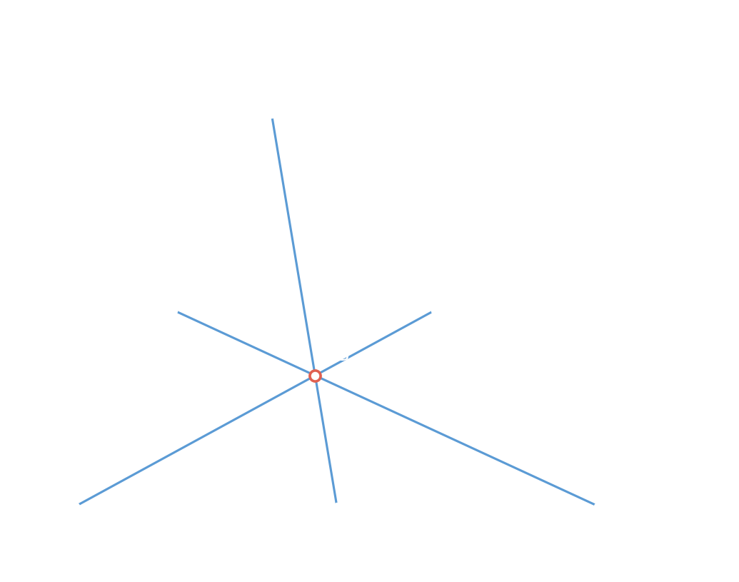
Theorem 12 (Concurrency of Medians)

The three medians of a triangle are concurrent. Their common point is called the centroid.

Proof

Let $ABC$ be a triangle with position vectors $\mathbf{a}, \mathbf{b}, \mathbf{c}$ . The midpoints of the sides $BC$ , $CA$ , $AB$ are, by Theorem 9:

\mathbf{d} = \frac{1}{2}(\mathbf{b}+\mathbf{c}), \qquad \mathbf{e} = \frac{1}{2}(\mathbf{c}+\mathbf{a}), \qquad \mathbf{f} = \frac{1}{2}(\mathbf{a}+\mathbf{b}).

Consider the median from $A$ to $D$ . By the parametric line equation (Theorem 11), any point on this median has position vector

\mathbf{x} = (1-t)\,\mathbf{a} + t\,\mathbf{d} = (1-t)\,\mathbf{a} + \frac{t}{2}(\mathbf{b}+\mathbf{c}).

Choosing $t = 2/3$ gives

\mathbf{g} = \frac{1}{3}\mathbf{a} + \frac{1}{3}\mathbf{b} + \frac{1}{3}\mathbf{c} = \frac{1}{3}(\mathbf{a}+\mathbf{b}+\mathbf{c}).

The expression $\frac{1}{3}(\mathbf{a}+\mathbf{b}+\mathbf{c})$ is completely symmetric in $\mathbf{a}$ , $\mathbf{b}$ , $\mathbf{c}$ . Repeating the calculation on the median from $B$ to $E$ with parameter $t = 2/3$ from $B$ :

(1-\tfrac{2}{3})\,\mathbf{b} + \tfrac{2}{3}\,\mathbf{e} = \frac{1}{3}\mathbf{b} + \frac{1}{3}(\mathbf{c}+\mathbf{a}) = \frac{1}{3}(\mathbf{a}+\mathbf{b}+\mathbf{c}) = \mathbf{g}.

The same holds for the median from $C$ to $F$ . Since $\mathbf{g}$ lies on all three medians, the medians are concurrent at $G$ , the centroid.

■

The medians of a triangle intersect at the centroid G, which divides each median in a 2:1 ratio

Remark

The parameter $t = 2/3$ tells us that the centroid lies two-thirds of the way from each vertex to the opposite midpoint. Equivalently, the centroid divides each median in a $2:1$ ratio, measured from vertex to midpoint.

Note (Symmetry of an Expression)

An expression in several variables is called symmetric if it is unchanged when the variables are permuted. The formula $\frac{1}{3}(\mathbf{a} + \mathbf{b} + \mathbf{c})$ treats $\mathbf{a}$ , $\mathbf{b}$ , and $\mathbf{c}$ identically: swapping any two of them produces the same result. This means that any property we derive for one variable automatically holds for the others. In the proof above, once we showed that $\mathbf{g}$ lies on the median from $A$ , the symmetric form of $\mathbf{g}$ guaranteed the same conclusion for the medians from $B$ and $C$ without repeating the calculation. This reasoning pattern, known as argument by symmetry, appears frequently throughout mathematics: if the setup treats several objects identically, a conclusion established for one must hold for all.

Example 12

Let $A = (0, 0)$ , $B = (6, 0)$ , $C = (3, 6)$ . The centroid is

G = \frac{1}{3}(0+6+3,\; 0+0+6) = (3, 2).

We verify: the midpoint of $BC$ is $D = (9/2, 3)$ . On the median $AD$ , the point with $t = 2/3$ is

\frac{1}{3}(0,0) + \frac{2}{3}(9/2, 3) = (3, 2) = G. \quad \checkmark

Problem 9

Let $A = (1, 1)$ , $B = (5, 3)$ , $C = (3, 7)$ . Compute the centroid $G$ and verify that $G$ divides the median from $C$ to the midpoint of $AB$ in a $2:1$ ratio.

Affine Dependence and Menelaus’ Theorem

To handle more advanced incidence theorems, we need a more flexible criterion for collinearity than linear dependence of displacement vectors. The following result characterises collinearity through a condition on position vectors directly.

Theorem 13 (Affine Dependence)

Three points $X, Y, Z$ with position vectors $\mathbf{x}, \mathbf{y}, \mathbf{z}$ are collinear if and only if there exist scalars $u, v, w$ , not all zero, such that

u\mathbf{x} + v\mathbf{y} + w\mathbf{z} = \mathbf{0} \quad \text{and} \quad u + v + w = 0.

Proof

Suppose $X, Y, Z$ are collinear. Then $Z$ lies on the line through $X$ and $Y$ , so by the parametric line equation (Theorem 11), $\mathbf{z} = (1-t)\mathbf{x} + t\mathbf{y}$ for some scalar $t$ . Rearranging:

(1-t)\mathbf{x} + t\mathbf{y} - \mathbf{z} = \mathbf{0}.

Setting $u = 1-t$ , $v = t$ , $w = -1$ , we have $u\mathbf{x} + v\mathbf{y} + w\mathbf{z} = \mathbf{0}$ and $u + v + w = (1-t) + t - 1 = 0$ . Since $w = -1 \neq 0$ , not all scalars are zero.

Conversely, suppose $u\mathbf{x} + v\mathbf{y} + w\mathbf{z} = \mathbf{0}$ and $u + v + w = 0$ with, say, $w \neq 0$ . Then $w = -(u+v)$ , so

u\mathbf{x} + v\mathbf{y} - (u+v)\mathbf{z} = \mathbf{0} \implies (u+v)\mathbf{z} = u\mathbf{x} + v\mathbf{y}.

Since $w \neq 0$ , we have $u + v \neq 0$ , so we can divide:

\mathbf{z} = \frac{u}{u+v}\mathbf{x} + \frac{v}{u+v}\mathbf{y}.

Setting $t = \frac{v}{u+v}$ gives $1 - t = \frac{u}{u+v}$ , so $\mathbf{z} = (1-t)\mathbf{x} + t\mathbf{y}$ . By Theorem 11, $Z$ lies on the line through $X$ and $Y$ .

■

We now apply this criterion to prove Menelaus’ theorem, one of the classical results in triangle geometry. We first need a notion that measures where a point falls on a line relative to two reference points.

Definition 12 (Directed Ratio)

Let $A$ and $B$ be distinct points. For any point $Z$ on the line $L_{AB}$ with $Z \neq B$ , the directed ratio of $Z$ relative to $A, B$ , denoted $\mathrm{dr}(A, B;\, Z)$ , is the unique scalar $r$ such that

\overrightarrow{AZ} = r\,\overrightarrow{ZB}.

Remark

If $Z$ lies between $A$ and $B$ , then $\overrightarrow{AZ}$ and $\overrightarrow{ZB}$ point in the same direction, so $r > 0$ . If $Z$ lies outside the segment $\overline{AB}$ , they point in opposite directions, so $r < 0$ . In terms of position vectors, $\mathbf{z} - \mathbf{a} = r(\mathbf{b} - \mathbf{z})$ , which rearranges to $(1+r)\mathbf{z} = \mathbf{a} + r\mathbf{b}$ .

Example 13

Let $A = (0, 0)$ and $B = (6, 0)$ . The point $Z = (2, 0)$ lies between $A$ and $B$ . We have $\overrightarrow{AZ} = \begin{bmatrix} 2 \\ 0 \end{bmatrix}$ and $\overrightarrow{ZB} = \begin{bmatrix} 4 \\ 0 \end{bmatrix}$ , so $\overrightarrow{AZ} = \frac{1}{2}\overrightarrow{ZB}$ and $\mathrm{dr}(A, B;\, Z) = 1/2 > 0$ . The point $Z' = (-3, 0)$ lies outside $\overline{AB}$ : $\overrightarrow{AZ'} = \begin{bmatrix} -3 \\ 0 \end{bmatrix}$ and $\overrightarrow{Z'B} = \begin{bmatrix} 9 \\ 0 \end{bmatrix}$ , so $\mathrm{dr}(A, B;\, Z') = -1/3 < 0$ .

Theorem 14 (Menelaus' Theorem)

Let $X, Y, Z$ be points on the lines containing sides $BC$ , $CA$ , $AB$ of a triangle $ABC$ , respectively. Then $X, Y, Z$ are collinear if and only if

\mathrm{dr}(B, C;\, X) \cdot \mathrm{dr}(C, A;\, Y) \cdot \mathrm{dr}(A, B;\, Z) = -1.

Proof

Let $r = \mathrm{dr}(B, C;\, X)$ , $s = \mathrm{dr}(C, A;\, Y)$ , and $t = \mathrm{dr}(A, B;\, Z)$ . From the definition of directed ratio:

(1+r)\mathbf{x} = \mathbf{b} + r\mathbf{c}, \qquad (1+s)\mathbf{y} = \mathbf{c} + s\mathbf{a}, \qquad (1+t)\mathbf{z} = \mathbf{a} + t\mathbf{b}.

Assume $rst = -1$ . We form a linear combination of $\mathbf{x}$ , $\mathbf{y}$ , $\mathbf{z}$ designed to satisfy the affine dependence criterion (Theorem 13). Consider

st(1+r)\,\mathbf{x} + (1+s)\,\mathbf{y} - s(1+t)\,\mathbf{z}.

Substituting the expressions above:

st(\mathbf{b} + r\mathbf{c}) + (\mathbf{c} + s\mathbf{a}) - s(\mathbf{a} + t\mathbf{b})

= st\mathbf{b} + str\mathbf{c} + \mathbf{c} + s\mathbf{a} - s\mathbf{a} - st\mathbf{b} = (str + 1)\mathbf{c}.

Since $rst = -1$ , we have $str + 1 = 0$ , so the entire combination equals $\mathbf{0}$ .

We also check the sum of the coefficients:

st(1+r) + (1+s) - s(1+t) = st + str + 1 + s - s - st = str + 1 = 0.

By Theorem 13, the points $X, Y, Z$ are collinear.

The converse follows by reversing the argument: if $X, Y, Z$ are collinear, Theorem 13 provides scalars $u, v, w$ with $u + v + w = 0$ and $u\mathbf{x} + v\mathbf{y} + w\mathbf{z} = \mathbf{0}$ . Expressing $\mathbf{x}, \mathbf{y}, \mathbf{z}$ in terms of $\mathbf{a}, \mathbf{b}, \mathbf{c}$ and comparing coefficients forces $rst = -1$ .

■

Menelaus' theorem: points X, Y, Z on the sides of triangle ABC are collinear

Example 14

Consider the triangle with $A = (0, 0)$ , $B = (4, 0)$ , $C = (3, 3)$ . Let the line $\ell$ intersect side $CA$ at $Y = (1.2,\, 1.2)$ and line $AB$ at $Z = (-1.5,\, 0)$ . We compute the directed ratios and verify Menelaus’ condition.

For $Y$ on $CA$ : $\overrightarrow{CY} = (-1.8,\, -1.8)$ and $\overrightarrow{YA} = (-1.2,\, -1.2)$ , so $s = \mathrm{dr}(C, A;\, Y) = 3/2$ .

For $Z$ on $AB$ : $\overrightarrow{AZ} = (-1.5,\, 0)$ and $\overrightarrow{ZB} = (5.5,\, 0)$ , so $t = \mathrm{dr}(A, B;\, Z) = -3/11$ .

Menelaus requires $r \cdot s \cdot t = -1$ , giving $r = -1/(st) = -1/((3/2)(-3/11)) = 22/9$ .

Problem 10

Let $A = (0, 0)$ , $B = (6, 0)$ , $C = (2, 4)$ . The point $X$ lies on $BC$ with $\mathrm{dr}(B, C;\, X) = 1$ (i.e., $X$ is the midpoint of $BC$ ), and $Z$ lies on line $AB$ with $\mathrm{dr}(A, B;\, Z) = -1/2$ . Use Menelaus’ theorem to find $\mathrm{dr}(C, A;\, Y)$ , and hence determine the coordinates of $Y$ on line $CA$ .

The Dot Product

In the preceding sections, we employed vector algebra to investigate affine properties of plane geometry: parallelism, collinearity, and ratios of segments. These properties are independent of any specific unit of measurement. However, to discuss metric geometry (concepts involving lengths and angles), we require a stronger algebraic tool. This tool is the dot product.

Definition 13 (Dot Product)

Let $\mathbf{a} = \begin{bmatrix} a_1 \\ a_2 \end{bmatrix}$ and $\mathbf{b} = \begin{bmatrix} b_1 \\ b_2 \end{bmatrix}$ be vectors in $\mathbb{R}^2$ . The dot product (also known as the scalar product or inner product) of $\mathbf{a}$ and $\mathbf{b}$ is the real number defined by:

\mathbf{a} \cdot \mathbf{b} = a_1 b_1 + a_2 b_2.

It is crucial to observe that while the operation takes two vectors as input, the output is a scalar. By examining the definition alongside our earlier definition of magnitude (Definition 3), we immediately observe a fundamental link between the dot product and the magnitude of a vector:

\mathbf{a} \cdot \mathbf{a} = a_1^2 + a_2^2 = |\mathbf{a}|^2.

Thus, the magnitude of a vector is the square root of the dot product of the vector with itself: $|\mathbf{a}| = \sqrt{\mathbf{a} \cdot \mathbf{a}}$ .

Example 15

Let $\mathbf{a} = \begin{bmatrix} 3 \\ -1 \end{bmatrix}$ and $\mathbf{b} = \begin{bmatrix} 2 \\ 4 \end{bmatrix}$ . Then $\mathbf{a} \cdot \mathbf{b} = (3)(2) + (-1)(4) = 2$ . Also, $\mathbf{a} \cdot \mathbf{a} = 9 + 1 = 10 = |\mathbf{a}|^2$ , consistent with $|\mathbf{a}| = \sqrt{10}$ from Definition 3.

The dot product satisfies several fundamental algebraic laws which justify its manipulation in equations.

Theorem 15 (Algebraic Properties of the Dot Product)

For any vectors $\mathbf{a}, \mathbf{b}, \mathbf{c} \in \mathbb{R}^2$ and any scalar $r \in \mathbb{R}$ , the following hold:

Symmetry: $\mathbf{a} \cdot \mathbf{b} = \mathbf{b} \cdot \mathbf{a}$ .
Bilinearity: The dot product is linear in both arguments:
- $(r\mathbf{a} + \mathbf{b}) \cdot \mathbf{c} = r(\mathbf{a} \cdot \mathbf{c}) + \mathbf{b} \cdot \mathbf{c}$ .
- $\mathbf{a} \cdot (r\mathbf{b} + \mathbf{c}) = r(\mathbf{a} \cdot \mathbf{b}) + \mathbf{a} \cdot \mathbf{c}$ .
Positive Definiteness: $\mathbf{a} \cdot \mathbf{a} \ge 0$ , with equality if and only if $\mathbf{a} = \mathbf{0}$ .

Proof

These properties follow directly from the properties of real numbers. Symmetry holds because $a_1 b_1 + a_2 b_2 = b_1 a_1 + b_2 a_2$ . Bilinearity is verified by expanding the components: $(ra_1 + b_1)c_1 + (ra_2 + b_2)c_2 = r(a_1 c_1 + a_2 c_2) + (b_1 c_1 + b_2 c_2)$ . The second bilinearity identity follows from symmetry and the first. Positive definiteness follows from the fact that $a_1^2 + a_2^2 \ge 0$ , with equality only when $a_1 = a_2 = 0$ .

■

Remark

The vector space $\mathbb{R}^2$ equipped with this specific dot product is often referred to as the Euclidean plane. This structure bridges the gap between abstract vector spaces and Euclidean geometry.

Metric Theorems

The interaction between the dot product and the magnitude leads to several powerful inequalities and identities.

Theorem 16 (Fundamental Metric Identities)

Let $\mathbf{a}$ and $\mathbf{b}$ be vectors in $\mathbb{R}^2$ .

Homogeneity: $|r\mathbf{a}| = |r|\,|\mathbf{a}|$ .
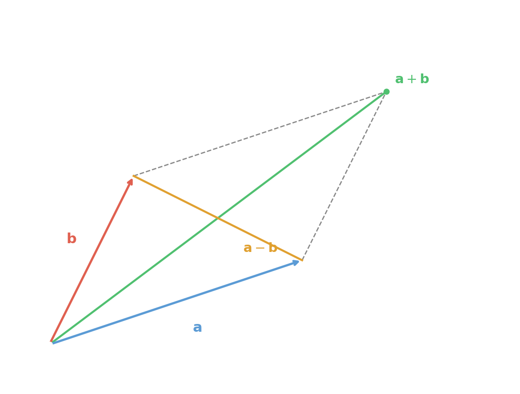
Parallelogram Law: $|\mathbf{a} + \mathbf{b}|^2 + |\mathbf{a} - \mathbf{b}|^2 = 2(|\mathbf{a}|^2 + |\mathbf{b}|^2)$ .
Cauchy-Schwarz Inequality: $|\mathbf{a} \cdot \mathbf{b}| \le |\mathbf{a}|\,|\mathbf{b}|$ .
Triangle Inequality: $|\mathbf{a} + \mathbf{b}| \le |\mathbf{a}| + |\mathbf{b}|$ .
Law of Cosines: $|\mathbf{a} - \mathbf{b}|^2 = |\mathbf{a}|^2 + |\mathbf{b}|^2 - 2(\mathbf{a} \cdot \mathbf{b})$ .

Proof

(i) We have $|r\mathbf{a}|^2 = (r\mathbf{a}) \cdot (r\mathbf{a}) = r^2(\mathbf{a} \cdot \mathbf{a}) = r^2 |\mathbf{a}|^2$ . Taking square roots gives $|r\mathbf{a}| = |r|\,|\mathbf{a}|$ .

(ii) We expand the norms using the dot product properties:

|\mathbf{a} + \mathbf{b}|^2 = (\mathbf{a} + \mathbf{b}) \cdot (\mathbf{a} + \mathbf{b}) = |\mathbf{a}|^2 + 2(\mathbf{a} \cdot \mathbf{b}) + |\mathbf{b}|^2

|\mathbf{a} - \mathbf{b}|^2 = (\mathbf{a} - \mathbf{b}) \cdot (\mathbf{a} - \mathbf{b}) = |\mathbf{a}|^2 - 2(\mathbf{a} \cdot \mathbf{b}) + |\mathbf{b}|^2

Adding these two equations yields the result. Geometrically, this states that the sum of the squares of the diagonals of a parallelogram equals the sum of the squares of its sides.

(iii) If $\mathbf{a} = \mathbf{0}$ , the inequality holds trivially. Assume $\mathbf{a} \neq \mathbf{0}$ . Consider the vector $\mathbf{v}(x) = x\mathbf{a} + \mathbf{b}$ for any scalar $x$ . By positive definiteness, $|\mathbf{v}(x)|^2 \ge 0$ . Expanding:

|x\mathbf{a} + \mathbf{b}|^2 = x^2|\mathbf{a}|^2 + 2x(\mathbf{a} \cdot \mathbf{b}) + |\mathbf{b}|^2 \ge 0.

This is a quadratic polynomial in $x$ . Since it is non-negative for all real $x$ , its discriminant must be non-positive:

\Delta = 4(\mathbf{a} \cdot \mathbf{b})^2 - 4|\mathbf{a}|^2 |\mathbf{b}|^2 \le 0 \implies (\mathbf{a} \cdot \mathbf{b})^2 \le |\mathbf{a}|^2 |\mathbf{b}|^2.

Taking the square root yields $|\mathbf{a} \cdot \mathbf{b}| \le |\mathbf{a}|\,|\mathbf{b}|$ .

(iv) Using the expansion from part (ii) and the Cauchy-Schwarz inequality:

|\mathbf{a} + \mathbf{b}|^2 = |\mathbf{a}|^2 + |\mathbf{b}|^2 + 2(\mathbf{a} \cdot \mathbf{b}) \le |\mathbf{a}|^2 + |\mathbf{b}|^2 + 2|\mathbf{a}|\,|\mathbf{b}| = (|\mathbf{a}| + |\mathbf{b}|)^2.

Taking square roots gives $|\mathbf{a} + \mathbf{b}| \le |\mathbf{a}| + |\mathbf{b}|$ .

(v) This is simply the expansion $|\mathbf{a} - \mathbf{b}|^2 = (\mathbf{a} - \mathbf{b}) \cdot (\mathbf{a} - \mathbf{b}) = |\mathbf{a}|^2 - 2(\mathbf{a} \cdot \mathbf{b}) + |\mathbf{b}|^2$ .

■

The Parallelogram Law involves the diagonals a+b and a-b

Angle and Orthogonality

To appreciate why identity (v) in Theorem 16 is commonly referred to as the Cosine Law for vectors, consider a triangle $OAB$ in the plane. Let $\theta$ be the angle at the vertex $O$ . The classical Law of Cosines from trigonometry states:

AB^2 = OA^2 + OB^2 - 2(OA)(OB)\cos\theta.

Setting $\mathbf{a} = \overrightarrow{OA}$ and $\mathbf{b} = \overrightarrow{OB}$ , we have $AB = |\mathbf{a} - \mathbf{b}|$ . Substituting:

|\mathbf{a} - \mathbf{b}|^2 = |\mathbf{a}|^2 + |\mathbf{b}|^2 - 2|\mathbf{a}|\,|\mathbf{b}|\cos\theta.

Comparing this with identity (v), which gives $|\mathbf{a} - \mathbf{b}|^2 = |\mathbf{a}|^2 + |\mathbf{b}|^2 - 2(\mathbf{a} \cdot \mathbf{b})$ , we equate the angle-dependent terms:

\mathbf{a} \cdot \mathbf{b} = |\mathbf{a}|\,|\mathbf{b}|\cos\theta \quad \text{or equivalently} \quad \cos\theta = \frac{\mathbf{a} \cdot \mathbf{b}}{|\mathbf{a}|\,|\mathbf{b}|}.

This allows us to define the angle between two vectors rigorously. For the definition to be valid, the ratio on the right must lie in $[-1, 1]$ . The Cauchy-Schwarz inequality (identity (iii)) guarantees exactly this:

-1 \le \frac{\mathbf{a} \cdot \mathbf{b}}{|\mathbf{a}|\,|\mathbf{b}|} \le 1.

Thus the value is always valid for the arccosine function.

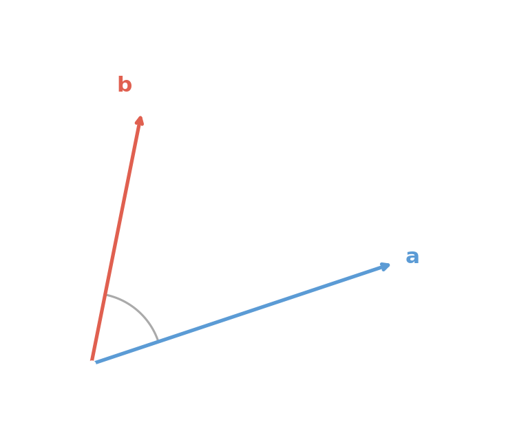
Definition 14 (Angle Between Vectors)

Let $\mathbf{a}$ and $\mathbf{b}$ be non-zero vectors. The angle $\theta$ between them is the unique number in the interval $[0, \pi]$ such that

\cos \theta = \frac{\mathbf{a} \cdot \mathbf{b}}{|\mathbf{a}|\,|\mathbf{b}|}.

The angle theta between vectors a and b is defined by their dot product

Example 16 (Calculating Angles)

Let $\mathbf{a} = \begin{bmatrix} 1 \\ 0 \end{bmatrix}$ , $\mathbf{b} = \begin{bmatrix} -1 \\ 1 \end{bmatrix}$ , and $\mathbf{c} = \begin{bmatrix} 5 \\ -5\sqrt{3} \end{bmatrix}$ . First, we compute the magnitudes: $|\mathbf{a}| = 1$ , $|\mathbf{b}| = \sqrt{2}$ , $|\mathbf{c}| = \sqrt{25 + 75} = 10$ .

(i) Angle between $\mathbf{a}$ and $\mathbf{b}$ : $\mathbf{a} \cdot \mathbf{b} = -1$ , so $\cos\theta = -1/\sqrt{2}$ , giving $\theta = 3\pi/4$ .

(ii) Angle between $\mathbf{a}$ and $\mathbf{c}$ : $\mathbf{a} \cdot \mathbf{c} = 5$ , so $\cos\theta = 5/10 = 1/2$ , giving $\theta = \pi/3$ .

(iii) Angle between $\mathbf{b}$ and $\mathbf{c}$ : $\mathbf{b} \cdot \mathbf{c} = -5 - 5\sqrt{3}$ , so $\cos\theta = -5(1+\sqrt{3})/(10\sqrt{2}) = -(\sqrt{2}+\sqrt{6})/4$ . This corresponds to $\theta = 11\pi/12$ .

The dot product also provides a simple algebraic test for perpendicularity. If vectors $\mathbf{a}$ and $\mathbf{b}$ are perpendicular, the angle between them is $\pi/2$ . Since $\cos(\pi/2) = 0$ , this implies $\mathbf{a} \cdot \mathbf{b} = 0$ . We formalise this as orthogonality, extending the concept to include the zero vector.

Definition 15 (Orthogonality)

Two vectors $\mathbf{a}$ and $\mathbf{b}$ are said to be orthogonal if $\mathbf{a} \cdot \mathbf{b} = 0$ . We denote this by $\mathbf{a} \perp \mathbf{b}$ .

Note

The zero vector is orthogonal to every vector in $\mathbb{R}^2$ , since $\mathbf{0} \cdot \mathbf{b} = 0$ for all $\mathbf{b}$ .

Example 17

The vectors $\mathbf{a} = \begin{bmatrix} 3 \\ 2 \end{bmatrix}$ and $\mathbf{b} = \begin{bmatrix} -2 \\ 3 \end{bmatrix}$ are orthogonal, since $\mathbf{a} \cdot \mathbf{b} = (3)(-2) + (2)(3) = 0$ . Notice that swapping the components and negating one always produces an orthogonal vector: if $\mathbf{a} = \begin{bmatrix} a_1 \\ a_2 \end{bmatrix}$ , then $\mathbf{a}^\perp = \begin{bmatrix} a_2 \\ -a_1 \end{bmatrix}$ satisfies $\mathbf{a} \cdot \mathbf{a}^\perp = a_1 a_2 - a_2 a_1 = 0$ .

Problem 11

Determine all vectors $\mathbf{b} = \begin{bmatrix} b_1 \\ b_2 \end{bmatrix}$ that are simultaneously orthogonal to $\mathbf{a} = \begin{bmatrix} 1 \\ 2 \end{bmatrix}$ and have magnitude $\sqrt{5}$ .

Orthogonal Projection

A fundamental problem in geometry and physics is the resolution of a vector into distinct components relative to a reference direction. Given a vector $\mathbf{x}$ and a non-zero reference vector $\mathbf{a}$ , we wish to decompose $\mathbf{x}$ into a sum $\mathbf{x} = \mathbf{p} + \mathbf{b}$ , where $\mathbf{p}$ is parallel to $\mathbf{a}$ and $\mathbf{b}$ is orthogonal to $\mathbf{a}$ .

One may approach this using elementary algebra. Let $\mathbf{a} = \begin{bmatrix} a_1 \\ a_2 \end{bmatrix} \neq \mathbf{0}$ . We seek a scalar $t$ and a scalar $u$ such that $\mathbf{x} = t\mathbf{a} + u\mathbf{a}^\perp$ , where $\mathbf{a}^\perp = \begin{bmatrix} a_2 \\ -a_1 \end{bmatrix}$ . This leads to the system:

a_1 t + a_2 u = x_1, \qquad a_2 t - a_1 u = x_2.

Multiplying the first equation by $a_1$ and the second by $a_2$ , then adding, eliminates $u$ :

(a_1^2 + a_2^2)\,t = a_1 x_1 + a_2 x_2.

Recognising the terms as dot products and magnitudes, we obtain $t\,|\mathbf{a}|^2 = \mathbf{x} \cdot \mathbf{a}$ , giving $t = (\mathbf{x} \cdot \mathbf{a})/|\mathbf{a}|^2$ . This algebraic result motivates the following vector-based formulation.

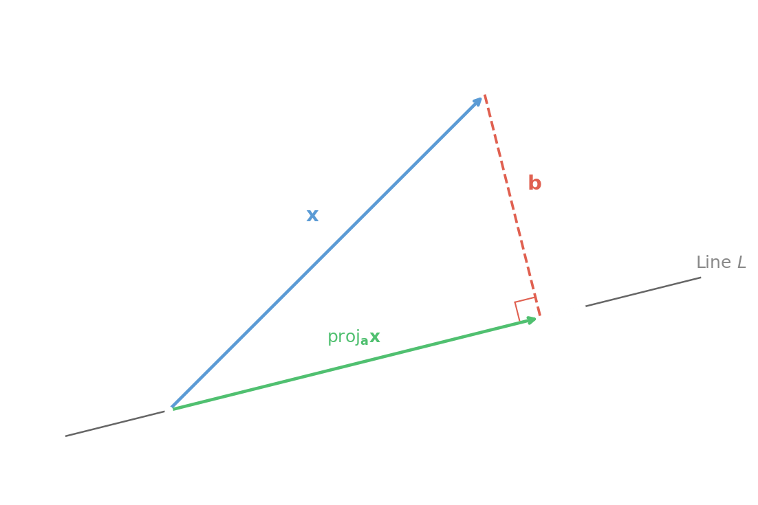
Theorem 17 (Orthogonal Decomposition)

Let $\mathbf{a} \in \mathbb{R}^2$ be a non-zero vector. For any vector $\mathbf{x} \in \mathbb{R}^2$ , there exists a unique scalar $t$ and a unique vector $\mathbf{b}$ such that

\mathbf{x} = t\mathbf{a} + \mathbf{b} \quad \text{and} \quad \mathbf{b} \perp \mathbf{a}.

The vector $\mathbf{p} = t\mathbf{a}$ is called the orthogonal projection of $\mathbf{x}$ onto $\mathbf{a}$ , denoted $\mathrm{proj}_{\mathbf{a}}\mathbf{x}$ .

Proof

We seek a scalar $t$ such that the vector $\mathbf{b} = \mathbf{x} - t\mathbf{a}$ is orthogonal to $\mathbf{a}$ :

(\mathbf{x} - t\mathbf{a}) \cdot \mathbf{a} = 0 \implies \mathbf{x} \cdot \mathbf{a} - t(\mathbf{a} \cdot \mathbf{a}) = 0.

Since $\mathbf{a} \neq \mathbf{0}$ , we have $\mathbf{a} \cdot \mathbf{a} \neq 0$ , yielding the unique solution:

t = \frac{\mathbf{x} \cdot \mathbf{a}}{\mathbf{a} \cdot \mathbf{a}} = \frac{\mathbf{x} \cdot \mathbf{a}}{|\mathbf{a}|^2}.

The projection vector is therefore:

\mathrm{proj}_{\mathbf{a}}\mathbf{x} = \left(\frac{\mathbf{x} \cdot \mathbf{a}}{|\mathbf{a}|^2}\right)\mathbf{a}.

■

Graphically, the term $\mathbf{b} = \mathbf{x} - \mathrm{proj}_{\mathbf{a}}\mathbf{x}$ represents the perpendicular distance from the tip of $\mathbf{x}$ to the line spanned by $\mathbf{a}$ .

The orthogonal decomposition of x onto the line generated by a

Corollary 1 (Special Cases)

$\mathbf{x}$ and $\mathbf{a}$ are linearly dependent if and only if $\mathrm{proj}_{\mathbf{a}}\mathbf{x} = \mathbf{x}$ (i.e., $\mathbf{b} = \mathbf{0}$ ).
$\mathbf{x}$ and $\mathbf{a}$ are orthogonal if and only if $\mathrm{proj}_{\mathbf{a}}\mathbf{x} = \mathbf{0}$ .

Proof

Recall from Theorem 17 that $\mathrm{proj}_{\mathbf{a}}\mathbf{x} = \left(\frac{\mathbf{x} \cdot \mathbf{a}}{|\mathbf{a}|^2}\right)\mathbf{a}$ and $\mathbf{b} = \mathbf{x} - \mathrm{proj}_{\mathbf{a}}\mathbf{x}$ .

(i) If $\mathbf{x}$ and $\mathbf{a}$ are linearly dependent, then $\mathbf{x} = k\mathbf{a}$ for some scalar $k$ . Then $\mathbf{x} \cdot \mathbf{a} = k|\mathbf{a}|^2$ , so $\mathrm{proj}_{\mathbf{a}}\mathbf{x} = k\mathbf{a} = \mathbf{x}$ , giving $\mathbf{b} = \mathbf{0}$ . Conversely, if $\mathrm{proj}_{\mathbf{a}}\mathbf{x} = \mathbf{x}$ , then $\mathbf{x} = \left(\frac{\mathbf{x} \cdot \mathbf{a}}{|\mathbf{a}|^2}\right)\mathbf{a}$ , which expresses $\mathbf{x}$ as a scalar multiple of $\mathbf{a}$ .

(ii) If $\mathbf{x} \perp \mathbf{a}$ , then $\mathbf{x} \cdot \mathbf{a} = 0$ , so $\mathrm{proj}_{\mathbf{a}}\mathbf{x} = \mathbf{0}$ . Conversely, if $\mathrm{proj}_{\mathbf{a}}\mathbf{x} = \mathbf{0}$ , then $\frac{\mathbf{x} \cdot \mathbf{a}}{|\mathbf{a}|^2} = 0$ , which implies $\mathbf{x} \cdot \mathbf{a} = 0$ , so $\mathbf{x} \perp \mathbf{a}$ .

■

The length of the projection vector is given by:

|\mathrm{proj}_{\mathbf{a}}\mathbf{x}| = \left|\frac{\mathbf{x} \cdot \mathbf{a}}{|\mathbf{a}|^2}\right| |\mathbf{a}| = \frac{|\mathbf{x} \cdot \mathbf{a}|}{|\mathbf{a}|}.

This formula is particularly useful for finding the distance between points projected onto a line.

Example 18 (Projection of a Segment)

Let $X = (-1, 3)$ , $Y = (3, 0)$ , $A = (2, 4)$ , and $B = (1, -2)$ . We wish to find the length of the orthogonal projection of the segment $XY$ onto the line passing through $A$ and $B$ .

The displacement vectors are $\mathbf{z} = \overrightarrow{XY} = \begin{bmatrix} 4 \\ -3 \end{bmatrix}$ and $\mathbf{c} = \overrightarrow{AB} = \begin{bmatrix} -1 \\ -6 \end{bmatrix}$ . The length of the projection of segment $XY$ onto line $AB$ is:

\frac{|\mathbf{z} \cdot \mathbf{c}|}{|\mathbf{c}|} = \frac{|(4)(-1) + (-3)(-6)|}{\sqrt{1 + 36}} = \frac{14}{\sqrt{37}}.

Problem 12

Let $\mathbf{a} = \begin{bmatrix} 1 \\ 2 \end{bmatrix}$ and $\mathbf{x} = \begin{bmatrix} 7 \\ 1 \end{bmatrix}$ . Compute $\mathrm{proj}_{\mathbf{a}}\mathbf{x}$ and the orthogonal component $\mathbf{b} = \mathbf{x} - \mathrm{proj}_{\mathbf{a}}\mathbf{x}$ . Verify that $\mathbf{b} \perp \mathbf{a}$ .

The Equation of a Straight Line

In elementary coordinate geometry, a straight line is defined as the locus of points $X = (x, y)$ satisfying a linear equation of the form

ax + by + c = 0,

where $a$ and $b$ are not both zero. By translating this algebraic constraint into the language of vectors, we uncover the geometric significance of the coefficients $a$ and $b$ .

The Point-Normal Form

Let $\mathbf{n} = \begin{bmatrix} a \\ b \end{bmatrix}$ and let $\mathbf{x} = \begin{bmatrix} x \\ y \end{bmatrix}$ be the position vector of a point $X$ . The linear term $ax + by$ is precisely the dot product $\mathbf{n} \cdot \mathbf{x}$ . Consequently, the equation of the line may be rewritten as

\mathbf{n} \cdot \mathbf{x} + c = 0.

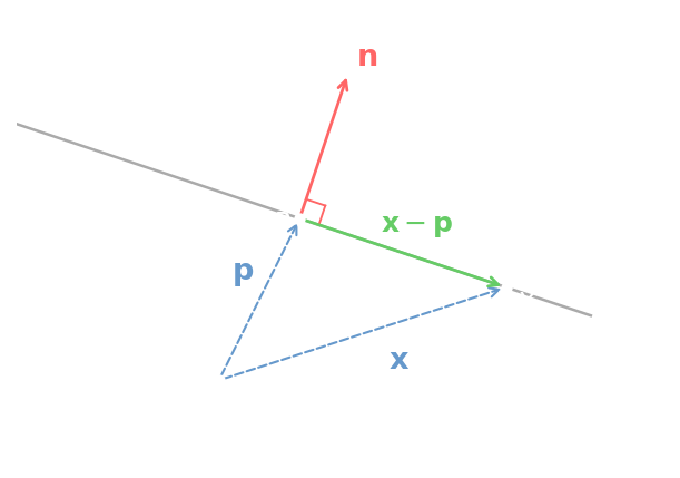
To interpret this geometrically, let $P$ be a fixed point on the line with position vector $\mathbf{p}$ . Since $P$ lies on the line, its coordinates satisfy the equation, so $\mathbf{n} \cdot \mathbf{p} + c = 0$ , which implies $c = -\mathbf{n} \cdot \mathbf{p}$ . Substituting this back into the general equation yields

\mathbf{n} \cdot \mathbf{x} - \mathbf{n} \cdot \mathbf{p} = 0 \implies \mathbf{n} \cdot (\mathbf{x} - \mathbf{p}) = 0.

The vector $\mathbf{x} - \mathbf{p}$ represents the displacement $\overrightarrow{PX}$ along the line. The condition $\mathbf{n} \cdot \overrightarrow{PX} = 0$ implies that $\mathbf{n}$ is orthogonal to the direction of the line.

Definition 16 (Normal Vector)

A non-zero vector $\mathbf{n}$ is called a normal vector to a straight line $L$ if $\mathbf{n}$ is orthogonal to the displacement vector between any two distinct points on $L$ .

This leads to the vector characterisation of a straight line.

Theorem 18 (Point-Normal Form)

The straight line passing through a specific point $P$ with position vector $\mathbf{p}$ , and perpendicular to a non-zero normal vector $\mathbf{n}$ , consists of all points $X$ with position vectors $\mathbf{x}$ satisfying

\mathbf{n} \cdot (\mathbf{x} - \mathbf{p}) = 0.

The line L through P with normal n, showing the displacement x minus p is orthogonal to n

Example 19 (Constructing a Line)

Find the equation of the line passing through $A(3, 2)$ and perpendicular to the vector $\mathbf{n} = \begin{bmatrix} 2 \\ -1 \end{bmatrix}$ .

Using the point-normal form:

\begin{bmatrix} 2 \\ -1 \end{bmatrix} \cdot \begin{bmatrix} x - 3 \\ y - 2 \end{bmatrix} = 0

2(x - 3) - 1(y - 2) = 0

2x - 6 - y + 2 = 0 \implies 2x - y - 4 = 0.

This formulation allows us to easily find the perpendicular bisector of a segment.

Example 20 (Perpendicular Bisector)

Let $A = (-1, 3)$ and $B = (5, 1)$ . The perpendicular bisector of $\overline{AB}$ passes through the midpoint $M$ of the segment and has $\overrightarrow{AB}$ as a normal vector.

Midpoint: $\mathbf{m} = \tfrac{1}{2}(\mathbf{a} + \mathbf{b}) = \begin{bmatrix} \frac{-1+5}{2} \\ \frac{3+1}{2} \end{bmatrix} = \begin{bmatrix} 2 \\ 2 \end{bmatrix}$ .
Normal vector: $\mathbf{n} = \mathbf{b} - \mathbf{a} = \begin{bmatrix} 6 \\ -2 \end{bmatrix}$ . For simplicity, we may use the parallel vector $\begin{bmatrix} 3 \\ -1 \end{bmatrix}$ .
Equation: $\begin{bmatrix} 3 \\ -1 \end{bmatrix} \cdot \begin{bmatrix} x - 2 \\ y - 2 \end{bmatrix} = 0 \implies 3(x - 2) - (y - 2) = 0 \implies 3x - y - 4 = 0$ .

Distance from a Point to a Line

The vector approach provides an elegant derivation for the distance from a point to a line, a result that is often tedious to prove using classical coordinates.

Theorem 19 (Distance to a Line)

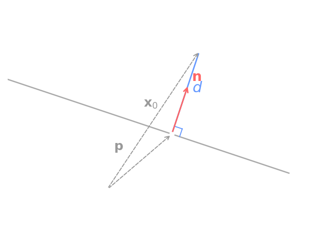
Let $L$ be the line defined by $\mathbf{n} \cdot \mathbf{x} + c = 0$ . The perpendicular distance from an arbitrary point $X_0$ (with position vector $\mathbf{x}_0$ ) to $L$ is given by

d(X_0, L) = \frac{|\mathbf{n} \cdot \mathbf{x}_0 + c|}{|\mathbf{n}|}.

Proof

Let $P$ be any point on the line $L$ . Then $\mathbf{n} \cdot \mathbf{p} + c = 0$ , so $c = -\mathbf{n} \cdot \mathbf{p}$ . The distance from $X_0$ to $L$ is the length of the orthogonal projection of the displacement vector $\overrightarrow{PX_0}$ onto the normal vector $\mathbf{n}$ .

Using the projection formula from Theorem 17:

d = |\mathrm{proj}_{\mathbf{n}}(\mathbf{x}_0 - \mathbf{p})| = \left|\left(\frac{(\mathbf{x}_0 - \mathbf{p}) \cdot \mathbf{n}}{|\mathbf{n}|^2}\right)\mathbf{n}\right| = \frac{|(\mathbf{x}_0 - \mathbf{p}) \cdot \mathbf{n}|}{|\mathbf{n}|}.

Expanding the dot product in the numerator:

d = \frac{|\mathbf{n} \cdot \mathbf{x}_0 - \mathbf{n} \cdot \mathbf{p}|}{|\mathbf{n}|}.

Substituting $-\mathbf{n} \cdot \mathbf{p} = c$ , we obtain

d = \frac{|\mathbf{n} \cdot \mathbf{x}_0 + c|}{|\mathbf{n}|}.

■

The distance d is the magnitude of the projection of the displacement onto the normal n

This theorem suggests a canonical way to represent straight lines. If we divide the equation $\mathbf{n} \cdot \mathbf{x} + c = 0$ by the magnitude $|\mathbf{n}|$ , we obtain the Hessian normal form:

\frac{\mathbf{n}}{|\mathbf{n}|} \cdot \mathbf{x} + \frac{c}{|\mathbf{n}|} = 0.

Defining the unit normal $\hat{\mathbf{n}} = \mathbf{n}/|\mathbf{n}|$ and $p = c/|\mathbf{n}|$ , the function $f(\mathbf{x}) = \hat{\mathbf{n}} \cdot \mathbf{x} + p$ has the property that $|f(\mathbf{x}_0)|$ gives the exact distance from $X_0$ to the line.

Example 21 (Distance Calculation)

Find the distance from $X_0(2, -1)$ to the line $3x + 4y - 12 = 0$ .

Here $\mathbf{n} = \begin{bmatrix} 3 \\ 4 \end{bmatrix}$ , so $|\mathbf{n}| = \sqrt{3^2 + 4^2} = 5$ .

d = \frac{|3(2) + 4(-1) - 12|}{5} = \frac{|6 - 4 - 12|}{5} = \frac{|-10|}{5} = 2.

Angle Between Lines

The angle between two straight lines is defined as the angle between their respective normal vectors. This definition is consistent with the geometric intuition that if two lines intersect, the angle between them is preserved if both are rotated by $90°$ (transforming the lines into their normals).

Theorem 20 (Angle Between Lines)

Let $L_1$ and $L_2$ be lines with normal vectors $\mathbf{n}_1$ and $\mathbf{n}_2$ respectively. The angle $\theta \in [0, \pi]$ between the lines is given by

\cos\theta = \frac{\mathbf{n}_1 \cdot \mathbf{n}_2}{|\mathbf{n}_1|\,|\mathbf{n}_2|}.

If we are interested in the acute angle $\phi$ between the lines, we take the absolute value of the right-hand side: $\cos\phi = \frac{|\mathbf{n}_1 \cdot \mathbf{n}_2|}{|\mathbf{n}_1|\,|\mathbf{n}_2|}$ .

Example 22 (Angle Between Two Lines)

Find the angle between the lines $x - 2y + 3 = 0$ and $3x + y - 5 = 0$ .

The normal vectors are $\mathbf{n}_1 = \begin{bmatrix} 1 \\ -2 \end{bmatrix}$ and $\mathbf{n}_2 = \begin{bmatrix} 3 \\ 1 \end{bmatrix}$ .

\mathbf{n}_1 \cdot \mathbf{n}_2 = (1)(3) + (-2)(1) = 1.

|\mathbf{n}_1| = \sqrt{5}, \quad |\mathbf{n}_2| = \sqrt{10}.

\cos\theta = \frac{1}{\sqrt{5}\,\sqrt{10}} = \frac{1}{\sqrt{50}} = \frac{1}{5\sqrt{2}}.

Problem 13

Find the equation of the line passing through $A(1, 4)$ with normal vector $\mathbf{n} = \begin{bmatrix} 3 \\ 2 \end{bmatrix}$ . Then compute the perpendicular distance from $B(5, -1)$ to this line.

Problem 14

Two lines are given by $2x + y - 1 = 0$ and $x - 3y + 5 = 0$ . Determine the acute angle between them.