16/03/2026

#Math#Vectors#Geometry

Video

Lesson assets

video link

CS50P Lecture 0: Functions, Variables

exercise

Exercise 2 PDF

Vectors and Geometry in Space

In Lesson 1AM we developed the algebra of vectors in the plane, and in Lesson 1PM we used that algebra to recover geometric facts about lines, distances, and loci. We now extend this framework to three-dimensional space. While the geometric complexity increases, the algebraic methods developed for the plane generalise naturally. In this chapter, we construct the vector space $\mathbb{R}^3$ and explore the fundamental interplay between algebraic equations and solid geometry.

Cartesian Coordinates in Space

To define the position of a point in space algebraically, we require a reference system consisting of three mutually perpendicular lines intersecting at a common point, which we designate as the origin $O$ . We assign a direction to each line, establishing them as the $x$ -axis, the $y$ -axis, and the $z$ -axis.

Orientation

Unlike the plane, where the relative orientation of axes is generally fixed by a counter-clockwise convention from $x$ to $y$ , three-dimensional space offers a choice of orientation. There are $3! = 6$ possible assignments of axes to three mutually orthogonal lines. These assignments partition into two distinct classes.

Right-Hand Systems: Assignments that can be continuously rotated into one another.
Left-Hand Systems: Assignments that are mirror images of the first group and cannot be reached via rigid rotation.

Definition 17 (Right-Hand Coordinate System)

A coordinate system is said to be right-handed if the $x$ , $y$ , and $z$ axes correspond respectively to the thumb, index finger, and middle finger of the right hand when extended in mutually perpendicular directions.

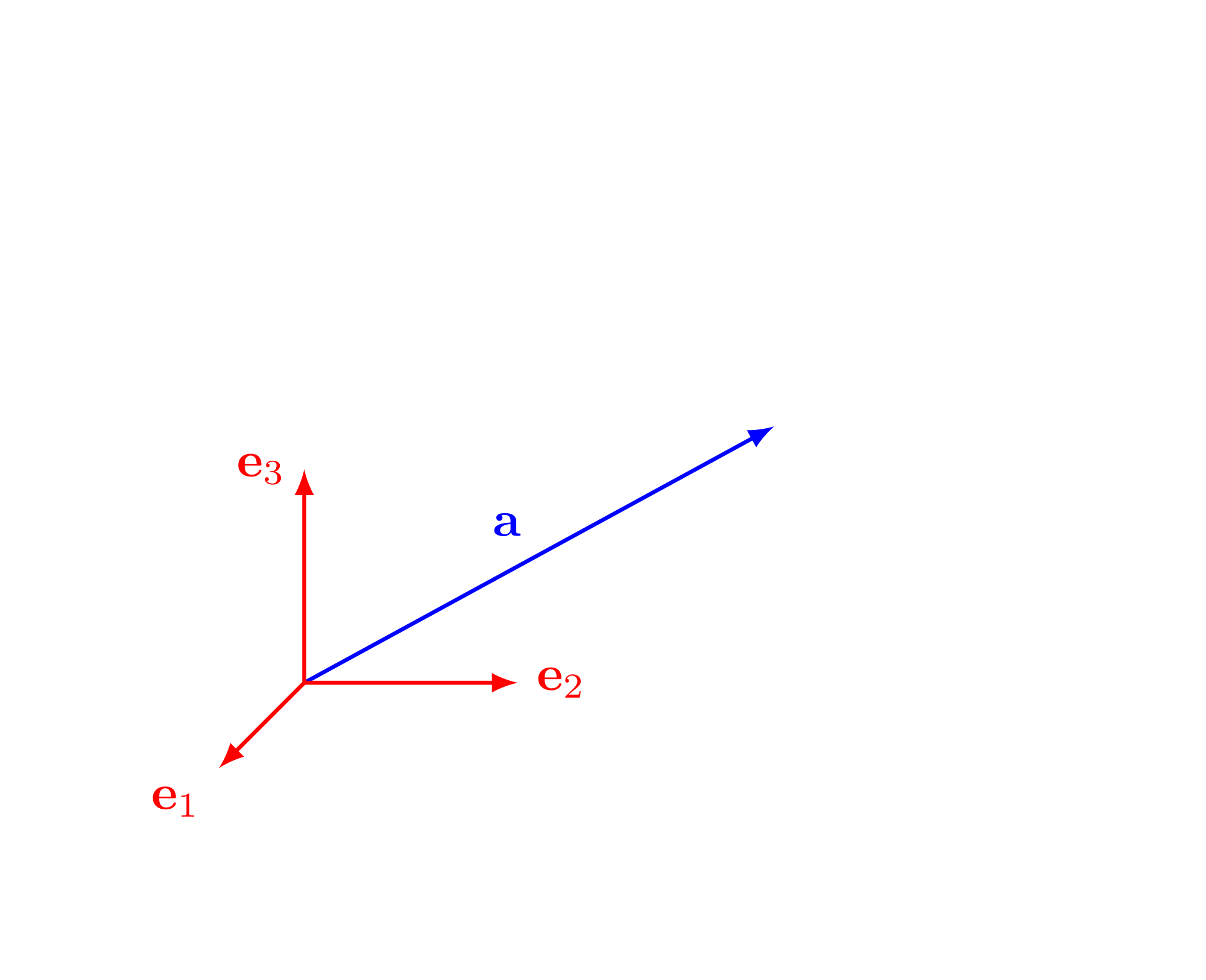
We shall exclusively adopt the right-hand coordinate system. This choice ensures consistency with standard conventions in physics and vector calculus, particularly regarding the cross product (to be discussed in subsequent sections). The following figure fixes the orientation we shall use throughout the chapter.

A right-handed coordinate system with mutually perpendicular x-, y-, and z-axes

The Bijection between Points and Triples

We identify each coordinate axis with the real line $\mathbb{R}$ . Given an ordered triple of real numbers $(a_1, a_2, a_3)$ , we associate it with a unique point $A$ in space via the intersection of three planes:

The plane perpendicular to the $x$ -axis at $a_1$ .
The plane perpendicular to the $y$ -axis at $a_2$ .
The plane perpendicular to the $z$ -axis at $a_3$ .

Conversely, for any point $B$ in space, we construct planes passing through $B$ perpendicular to the axes, intersecting them at coordinates $b_1, b_2, b_3$ respectively. This establishes a one-to-one correspondence between solid geometry and algebra.

Definition 18 (Space Coordinates)

The ordered triple of real numbers $(a_1, a_2, a_3)$ associated with a point $A$ are called the coordinates of $A$ . We write $A = (a_1, a_2, a_3)$ . The set of all such ordered triples is denoted by $\mathbb{R}^3$ .

The point A with coordinates a1, a2, a3 determined by three coordinate planes and the edges of a cuboid

Remark (Point and Vector)

As in Lesson 1AM, the same list of real numbers may appear either as a point or as a vector. The point $A = (a_1, a_2, a_3)$ is a location in space, whereas the vector $\mathbf{a} = \begin{bmatrix} a_1 \\ a_2 \\ a_3 \end{bmatrix}$ is a displacement. The algebra is the same component-wise; the geometric role is not.

Example 23 (Locating a Point in Space)

Fix the origin at a survey marker on the ground. Let the positive $x$ -axis point due east, the positive $y$ -axis due north, and the positive $z$ -axis vertically upward. If a light fixed to a crane is $40$ metres east of the marker, $15$ metres south of it, and $18$ metres above the ground, then its position is recorded by the triple

(40, -15, 18).

If the same light is moved to a point $12$ metres west of the marker while retaining the same north-south and vertical displacements, then its coordinates become

(-12, -15, 18).

Thus the signs of the coordinates record on which side of each coordinate plane the point lies, and the ordered triple specifies the position completely.

Example 24 (Identifying Points in Space)

Consider a cube of side length $2$ resting in the first octant (where all coordinates are positive). One vertex is positioned at the origin $O = (0, 0, 0)$ , and the adjacent edges lie along the positive coordinate axes. The vertex diametrically opposite to the origin is found by translating $2$ units along the $x$ -axis, $2$ units along the $y$ -axis, and $2$ units along the $z$ -axis. Thus, its coordinates are $(2, 2, 2)$ .

The Euclidean Metric in Space

The metric properties of space are derived directly from the coordinate definitions by iteratively applying Pythagoras’ theorem. Just as distance in $\mathbb{R}^2$ requires a single application of the theorem, distance in $\mathbb{R}^3$ requires two.

Theorem 21 (Distance Formula in

\mathbb{R}^3

)

Let $A = (a_1, a_2, a_3)$ and $B = (b_1, b_2, b_3)$ be points in space. The Euclidean distance between $A$ and $B$ , denoted $|AB|$ , is given by

|AB| = \sqrt{(a_1 - b_1)^2 + (a_2 - b_2)^2 + (a_3 - b_3)^2}.

Proof

Let $A = (a_1, a_2, a_3)$ and $B = (b_1, b_2, b_3)$ . Consider the auxiliary point $C = (b_1, b_2, a_3)$ .

The points $A$ and $C$ both lie in the horizontal plane $z = a_3$ . Within this plane, the distance between them is determined by the planar distance formula:

|AC|^2 = (a_1 - b_1)^2 + (a_2 - b_2)^2.

The points $C$ and $B$ share the same $x$ and $y$ coordinates, meaning the segment $CB$ is parallel to the $z$ -axis. The length of this vertical segment is precisely $|a_3 - b_3|$ .

Because the segment $CB$ is orthogonal to the plane $z = a_3$ , it is orthogonal to any line within that plane, including the segment $AC$ . Therefore, the triangle $ACB$ is right-angled at $C$ . Applying Pythagoras’ theorem to this triangle yields:

|AB|^2 = |AC|^2 + |CB|^2 = \left( (a_1 - b_1)^2 + (a_2 - b_2)^2 \right) + (a_3 - b_3)^2.

Taking the positive square root completes the proof.

■

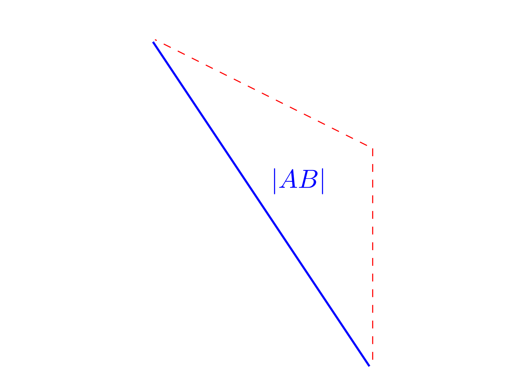
The next figure isolates the planar diagonal $AC$ and the vertical edge $CB$ used in the proof.

A cuboid showing points A, B, and C, where AC is a planar diagonal, CB is vertical, and AB is the space diagonal

If $B = O = (0, 0, 0)$ , the distance formula becomes

|OA| = \sqrt{a_1^2 + a_2^2 + a_3^2}.

This is the direct spatial analogue of the magnitude formula from Lesson 1AM.

Example 25 (Distance Computation)

Find the exact distance between the points $P = (1, -2, 4)$ and $Q = (3, 1, -2)$ .

Applying the distance formula:

|PQ| = \sqrt{(3 - 1)^2 + (1 - (-2))^2 + (-2 - 4)^2}

|PQ| = \sqrt{2^2 + 3^2 + (-6)^2} = \sqrt{4 + 9 + 36} = \sqrt{49} = 7.

The points are exactly $7$ units apart.

The Equation of a Sphere

The distance formula allows us to characterise geometric loci in space algebraically. The most fundamental of these is the sphere, perfectly mirroring the definition of a circle in the plane.

Definition 19 (Sphere)

A sphere is the locus of all points in space at a fixed distance $r$ (the radius) from a fixed point $C$ (the centre).

Let the centre be $C = (c_1, c_2, c_3)$ and let $X = (x, y, z)$ be an arbitrary point on the sphere. By definition, the distance is $|CX| = r$ . Squaring both sides and applying the distance formula, we obtain the standard equation of a sphere:

(x - c_1)^2 + (y - c_2)^2 + (z - c_3)^2 = r^2.

If an equation is given in an expanded polynomial form, we recover the geometric properties of the sphere by completing the square for each variable independently.

Example 26 (Spherical Equation)

Determine the set of points in $\mathbb{R}^3$ satisfying the equation:

x^2 + y^2 + z^2 - 2x - 4y + 6z - 11 = 0.

We collect the terms for each variable and complete the square:

(x^2 - 2x) + (y^2 - 4y) + (z^2 + 6z) = 11.

Adding the necessary constants to both sides:

(x^2 - 2x + 1) + (y^2 - 4y + 4) + (z^2 + 6z + 9) = 11 + 1 + 4 + 9.

Factoring the perfect squares gives:

(x - 1)^2 + (y - 2)^2 + (z + 3)^2 = 25.

This represents a sphere centred at $C = (1, 2, -3)$ with a radius of $r = \sqrt{25} = 5$ .

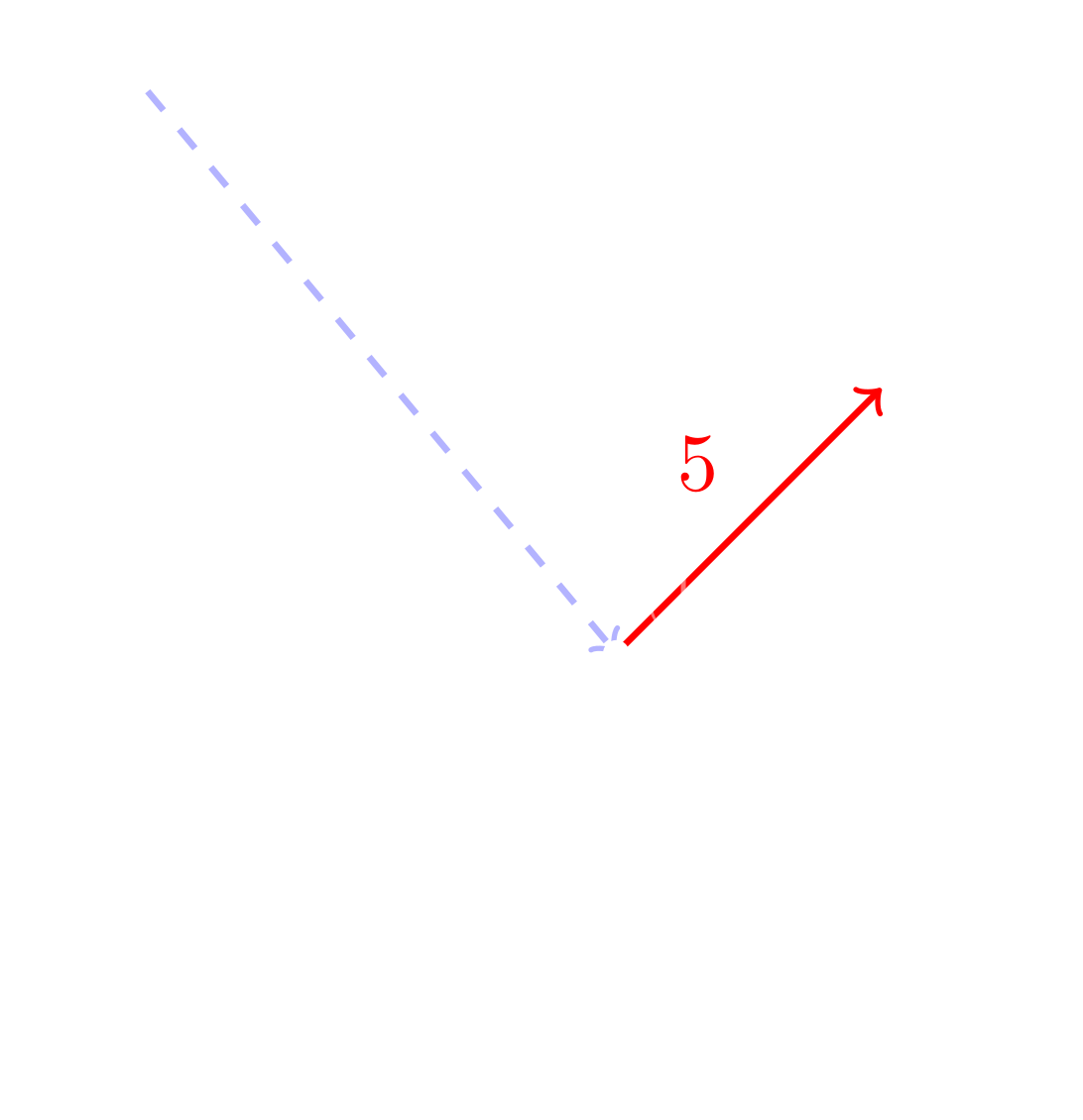
The following figure shows the centre and one radius for this sphere.

A sphere centred at C with a radius drawn to a point on the surface

Example 27 (Checking Whether a Point Lies on a Sphere)

Consider the sphere

x^2 + y^2 + z^2 = 9.

Its centre is the origin and its radius is $3$ . To test whether a point lies on the sphere, we substitute its coordinates into the equation.

For $(2, 1, 2)$ , we obtain

2^2 + 1^2 + 2^2 = 4 + 1 + 4 = 9,

so the point lies on the sphere.

For $(2, 2, 2)$ , we obtain

2^2 + 2^2 + 2^2 = 4 + 4 + 4 = 12 \neq 9,

so this point does not lie on the sphere.

Problem 17

A sphere passes through the origin and has its centre at the point $(3, -4, 1)$ . Determine the equation of the sphere and find the coordinates of the point diametrically opposite to the origin.

Problem 18

Determine whether the point $(3, -1, 2)$ lies on the sphere centred at $(1, -1, 0)$ with radius $2\sqrt{2}$ .

Vectors in Space

The passage from the Cartesian plane to space replaces coordinate pairs with ordered triples. Algebraically, very little changes. Geometrically, however, we now work with directed segments in three dimensions rather than in the plane.

Definition 20 (Vector in Space)

A vector in space is an ordered triple of real numbers, written as a column. The individual numbers are called the components of the vector. The set of all such vectors is denoted by $\mathbb{R}^3$ . Thus, a vector $\mathbf{a} \in \mathbb{R}^3$ is given by

\mathbf{a} = \begin{bmatrix} a_1 \\ a_2 \\ a_3 \end{bmatrix}.

As in Lesson 1AM, we keep the distinction between points and vectors strict. The ordered triple $(a_1, a_2, a_3)$ specifies the point $A$ , whereas the column $\mathbf{a}$ denotes a vector. The same three real numbers appear in both places, but their meanings are not interchangeable.

Geometrically, the vector $\mathbf{a}$ is represented by the directed segment from the origin $O=(0,0,0)$ to the point $A=(a_1,a_2,a_3)$ . In that situation, $\mathbf{a}$ is the position vector of $A$ . This is exactly the same idea as in the plane, only now a third component records vertical displacement as well.

Three vectors play a distinguished role. They record unit motion along the three coordinate axes:

\mathbf{e}_1 = \begin{bmatrix} 1 \\ 0 \\ 0 \end{bmatrix}, \qquad \mathbf{e}_2 = \begin{bmatrix} 0 \\ 1 \\ 0 \end{bmatrix}, \qquad \mathbf{e}_3 = \begin{bmatrix} 0 \\ 0 \\ 1 \end{bmatrix}.

The zero vector is

\mathbf{0} = \begin{bmatrix} 0 \\ 0 \\ 0 \end{bmatrix},

and corresponds to the degenerate directed segment at the origin.

Every vector in space is built from these three basis vectors in the evident way:

\mathbf{a} = \begin{bmatrix} a_1 \\ a_2 \\ a_3 \end{bmatrix} = a_1\mathbf{e}_1 + a_2\mathbf{e}_2 + a_3\mathbf{e}_3.

So the components of $\mathbf{a}$ are precisely the coefficients of $\mathbf{e}_1$ , $\mathbf{e}_2$ , and $\mathbf{e}_3$ in this decomposition.

The position vector a together with the standard basis vectors e1, e2, and e3 in R3

Example 28 (Decomposing a Vector in the Standard Basis)

Let

\mathbf{a} = \begin{bmatrix} 2 \\ -1 \\ 3 \end{bmatrix}.

Then

\mathbf{a} = 2\mathbf{e}_1 - \mathbf{e}_2 + 3\mathbf{e}_3.

This says that to reach the endpoint of $\mathbf{a}$ from the origin, we move $2$ units in the $\mathbf{e}_1$ direction, $1$ unit in the opposite $\mathbf{e}_2$ direction, and $3$ units in the $\mathbf{e}_3$ direction.

The length of the directed segment representing $\mathbf{a}$ is its magnitude. Since the distance from the origin to $(a_1,a_2,a_3)$ was computed above, the definition is immediate.

Definition 21 (Magnitude in Space)

The magnitude (or norm) of a vector $\mathbf{a} = \begin{bmatrix} a_1 \\ a_2 \\ a_3 \end{bmatrix}$ is the non-negative real number

\|\mathbf{a}\| = \sqrt{a_1^2 + a_2^2 + a_3^2}.

Exactly as in the planar case, the zero vector is the unique vector with zero magnitude. Thus $\|\mathbf{a}\|=0$ if and only if $\mathbf{a}=\mathbf{0}$ .

Example 29 (Computing Magnitude)

Let

\mathbf{v} = \begin{bmatrix} 2 \\ -3 \\ 6 \end{bmatrix}.

Then

\|\mathbf{v}\| = \sqrt{2^2 + (-3)^2 + 6^2} = \sqrt{4 + 9 + 36} = \sqrt{49} = 7.

The Vector Space $\mathbb{R}^3$

Points in space are geometric locations. They are not added or scaled as points. Vectors, however, are algebraic objects, and the operations from Lesson 1AM extend component-wise without any change in principle.

Definition 22 (Operations in

\mathbb{R}^3

)

Let

\mathbf{a} = \begin{bmatrix} a_1 \\ a_2 \\ a_3 \end{bmatrix}, \qquad \mathbf{b} = \begin{bmatrix} b_1 \\ b_2 \\ b_3 \end{bmatrix},

and let $r \in \mathbb{R}$ .

The vector sum is

\mathbf{a} + \mathbf{b} = \begin{bmatrix} a_1 + b_1 \\ a_2 + b_2 \\ a_3 + b_3 \end{bmatrix}.

The scalar multiple is

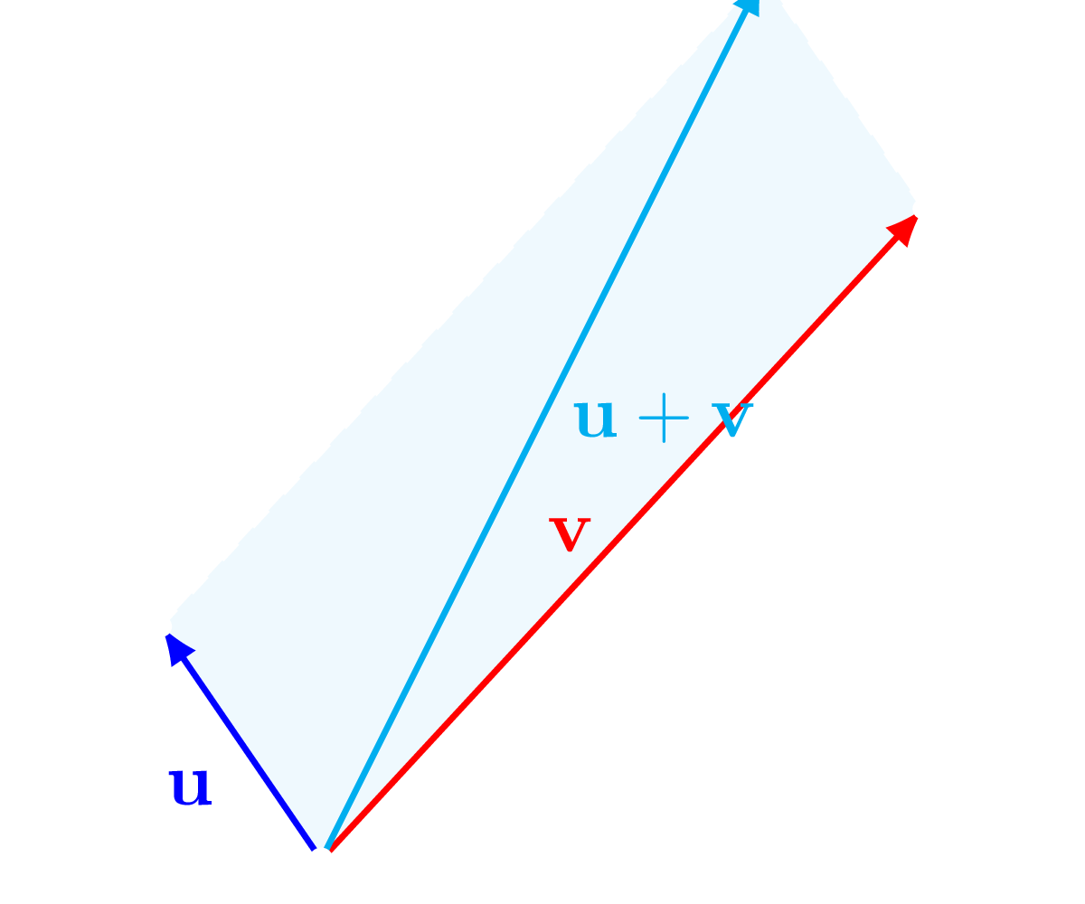
r\mathbf{a} = \begin{bmatrix} ra_1 \\ ra_2 \\ ra_3 \end{bmatrix}.

Geometrically, $\mathbf{a}+\mathbf{b}$ is still the diagonal of the parallelogram generated by $\mathbf{a}$ and $\mathbf{b}$ . The only new feature is that this parallelogram now lies in a plane sitting inside $\mathbb{R}^3$ rather than in the ambient space itself.

For example, let

\mathbf{u} = \begin{bmatrix} 3 \\ 1 \\ 2 \end{bmatrix}, \qquad \mathbf{v} = \begin{bmatrix} 1 \\ 3 \\ 3 \end{bmatrix}.

Then

\mathbf{u} + \mathbf{v} = \begin{bmatrix} 4 \\ 4 \\ 5 \end{bmatrix}.

The following figure shows the plane determined by $\mathbf{u}$ , $\mathbf{v}$ , and the origin. As in the planar case, the diagonal of the corresponding parallelogram is the sum vector.

Vectors u and v in space together with the parallelogram they determine and the diagonal u plus v

Example 30 (Linear Combinations in Space)

Let

\mathbf{a} = \begin{bmatrix} 1 \\ -2 \\ 0 \end{bmatrix}, \qquad \mathbf{b} = \begin{bmatrix} 3 \\ 1 \\ 4 \end{bmatrix}.

Then

2\mathbf{a} - \mathbf{b} = 2\begin{bmatrix} 1 \\ -2 \\ 0 \end{bmatrix} - \begin{bmatrix} 3 \\ 1 \\ 4 \end{bmatrix} = \begin{bmatrix} 2 \\ -4 \\ 0 \end{bmatrix} - \begin{bmatrix} 3 \\ 1 \\ 4 \end{bmatrix} = \begin{bmatrix} -1 \\ -5 \\ -4 \end{bmatrix}.

The set of all ordered triples, equipped with these two operations, is the vector space $\mathbb{R}^3$ . Its algebraic laws are the same as those of $\mathbb{R}^2$ .

Theorem 22 (Properties of

\mathbb{R}^3

)

Let $\mathbf{a}, \mathbf{b}, \mathbf{c}$ be vectors in $\mathbb{R}^3$ and let $r, s$ be scalars. Then:

$\mathbf{a} + \mathbf{b} = \mathbf{b} + \mathbf{a}$
$(\mathbf{a} + \mathbf{b}) + \mathbf{c} = \mathbf{a} + (\mathbf{b} + \mathbf{c})$
There exists a unique vector $\mathbf{0}$ such that $\mathbf{a} + \mathbf{0} = \mathbf{a}$ .
For every $\mathbf{a}$ , there exists a unique vector $-\mathbf{a}$ such that $\mathbf{a} + (-\mathbf{a}) = \mathbf{0}$ .
$(rs)\mathbf{a} = r(s\mathbf{a})$
$(r+s)\mathbf{a} = r\mathbf{a} + s\mathbf{a}$
$r(\mathbf{a} + \mathbf{b}) = r\mathbf{a} + r\mathbf{b}$
$1\mathbf{a} = \mathbf{a}$

Proof

These identities are checked component-wise, using only the algebraic laws of the real numbers. For example,

(rs)\mathbf{a} = \begin{bmatrix} (rs)a_1 \\ (rs)a_2 \\ (rs)a_3 \end{bmatrix} = \begin{bmatrix} r(sa_1) \\ r(sa_2) \\ r(sa_3) \end{bmatrix} = r\begin{bmatrix} sa_1 \\ sa_2 \\ sa_3 \end{bmatrix} = r(s\mathbf{a}).

All other properties are proved in exactly the same way.

■

Any theorem proved purely from these vector space axioms carries over from $\mathbb{R}^2$ to $\mathbb{R}^3$ without alteration. A basic instance is the zero product law.

Theorem 23 (Zero Product Law in Space)

Let $\mathbf{a} \in \mathbb{R}^3$ and let $r \in \mathbb{R}$ . Then $r\mathbf{a} = \mathbf{0}$ if and only if $r=0$ or $\mathbf{a}=\mathbf{0}$ .

Proof

The proof is identical to the axiomatic proof from Lesson 1AM. Only the vector space laws are used, and those laws are the same in $\mathbb{R}^3$ as in $\mathbb{R}^2$ .

■

Problem 19

Let

\mathbf{u} = \begin{bmatrix} 2 \\ t \\ -1 \end{bmatrix}, \qquad \mathbf{v} = \begin{bmatrix} 4 \\ 6 \\ s \end{bmatrix}.

Determine the values of $t$ and $s$ such that $\mathbf{v} = 2\mathbf{u}$ . Are $\mathbf{u}$ and $\mathbf{v}$ linearly dependent?

Linear Combinations and Independence

The concept of linear combinations, introduced in Lesson 1AM, extends naturally to $\mathbb{R}^3$ . This generalisation forms the foundation for understanding dimension and basis in higher-dimensional vector spaces. What changes is not the algebra but the geometry recovered from it: one vector generates a line through the origin, two suitably placed vectors generate a plane through the origin, and three suitably placed vectors may generate the whole space.

Definition 23 (Linear Combination)

Let $\mathbf{v}_1, \mathbf{v}_2, \dots, \mathbf{v}_k$ be vectors in $\mathbb{R}^3$ and let $c_1, c_2, \dots, c_k$ be scalars. The vector $\mathbf{v}$ defined by

\mathbf{v} = c_1\mathbf{v}_1 + c_2\mathbf{v}_2 + \dots + c_k\mathbf{v}_k

is called a linear combination of the vectors $\mathbf{v}_1, \dots, \mathbf{v}_k$ .

If $\mathbf{a} \neq \mathbf{0}$ , then the vectors $r\mathbf{a}$ form the line through the origin in the direction of $\mathbf{a}$ . If $\mathbf{a}$ and $\mathbf{b}$ are not scalar multiples of one another, then the vectors $r\mathbf{a} + s\mathbf{b}$ form the plane through the origin spanned by $\mathbf{a}$ and $\mathbf{b}$ .

Example 31 (A Plane Obtained from Linear Combinations)

Take

\mathbf{a} = \mathbf{e}_1 = \begin{bmatrix} 1 \\ 0 \\ 0 \end{bmatrix}, \qquad \mathbf{b} = \mathbf{e}_2 = \begin{bmatrix} 0 \\ 1 \\ 0 \end{bmatrix}.

Then

r\mathbf{a} + s\mathbf{b} = \begin{bmatrix} r \\ 0 \\ 0 \end{bmatrix} + \begin{bmatrix} 0 \\ s \\ 0 \end{bmatrix} = \begin{bmatrix} r \\ s \\ 0 \end{bmatrix}.

So the linear combinations of $\mathbf{e}_1$ and $\mathbf{e}_2$ are precisely the vectors lying in the plane $z=0$ .

Linear Independence of Two Vectors

The definition of linear independence for two vectors in space is the same as in the planar case.

Definition 24 (Independence of Two Vectors)

Two vectors $\mathbf{a}, \mathbf{b} \in \mathbb{R}^3$ are linearly independent if neither is a scalar multiple of the other. If one is a scalar multiple of the other, they are linearly dependent.

We establish four equivalent conditions for linear dependence in space. Observe the expansion of the algebraic determinant condition compared to its planar counterpart.

Theorem 24 (Conditions for Linear Dependence of Two Vectors)

Let $\mathbf{a} = \begin{bmatrix} a_1 \\ a_2 \\ a_3 \end{bmatrix}$ and $\mathbf{b} = \begin{bmatrix} b_1 \\ b_2 \\ b_3 \end{bmatrix}$ . The following statements are equivalent:

$\mathbf{a}$ and $\mathbf{b}$ are linearly dependent.
The points $O(0,0,0)$ , $A(a_1, a_2, a_3)$ , and $B(b_1, b_2, b_3)$ are collinear.
There exist scalars $r$ and $s$ , not both zero, such that $r\mathbf{a} + s\mathbf{b} = \mathbf{0}$ .
$a_1 b_2 - a_2 b_1 = 0, \quad a_2 b_3 - a_3 b_2 = 0, \quad \text{and} \quad a_3 b_1 - a_1 b_3 = 0$ .

Proof

The equivalence of statements 1, 2, and 3 is proved exactly as in the plane. We therefore only check the equivalence of 1 and 4.

Assume statement 1 holds. Without loss of generality, let $\mathbf{a} = r\mathbf{b}$ . Then $a_i = r b_i$ for $i=1,2,3$ . Substituting into the first expression of 4:

a_1 b_2 - a_2 b_1 = (r b_1)b_2 - (r b_2)b_1 = r(b_1 b_2 - b_2 b_1) = 0.

By symmetry, the other two expressions also vanish.

Conversely, assume statement 4 holds. If $\mathbf{b} = \mathbf{0}$ , dependence is immediate. If $\mathbf{b} \neq \mathbf{0}$ , choose an index $i$ for which $b_i \neq 0$ . If $i=1$ , let $r = a_1/b_1$ . Then

a_1 b_2 - a_2 b_1 = 0 \quad \text{and} \quad a_3 b_1 - a_1 b_3 = 0

give

a_2 = \frac{a_1}{b_1} b_2 = rb_2, \qquad a_3 = \frac{a_1}{b_1} b_3 = rb_3.

Hence $\mathbf{a} = r\mathbf{b}$ . The cases $i=2$ and $i=3$ are handled in the same way. Thus statement 4 implies statement 1.

■

Note (Cross Product Preview)

Condition 4 requires that all three $2 \times 2$ determinants formed by the coordinate pairs of $\mathbf{a}$ and $\mathbf{b}$ must vanish simultaneously. This algebraic requirement directly anticipates the cross product; specifically, two vectors in space are linearly dependent if and only if their cross product is the zero vector.

By negating the previous theorem, we obtain the corresponding criterion for independence.

Theorem 25 (Conditions for Linear Independence of Two Vectors)

Let $\mathbf{a}, \mathbf{b} \in \mathbb{R}^3$ . The following statements are equivalent:

$\mathbf{a}$ and $\mathbf{b}$ are linearly independent.
The points $O, A, B$ are distinct and not collinear.
The equation $r\mathbf{a} + s\mathbf{b} = \mathbf{0}$ implies $r = 0$ and $s = 0$ .
At least one of the expressions $a_1 b_2 - a_2 b_1$ , $a_2 b_3 - a_3 b_2$ , or $a_3 b_1 - a_1 b_3$ is non-zero.

Proof

Each statement here is the logical negation of the corresponding statement in the preceding dependence theorem.

■

Linear Independence of Three Vectors

The third dimension naturally permits the simultaneous consideration of three vectors.

Definition 25 (Independence of Three Vectors)

Three vectors $\mathbf{a}, \mathbf{b}, \mathbf{c} \in \mathbb{R}^3$ are linearly dependent if at least one of them can be expressed as a linear combination of the other two. They are linearly independent if none is a linear combination of the others.

The standard basis vectors $\mathbf{e}_1, \mathbf{e}_2, \mathbf{e}_3$ constitute a primary example of three linearly independent vectors. The algebraic criterion for their dependence relies on finding a non-trivial linear combination that yields the zero vector.

Theorem 26 (Algebraic Criterion for Three Vectors)

Three vectors $\mathbf{a}, \mathbf{b}, \mathbf{c}$ are linearly dependent if and only if there exist scalars $r, s, t$ , not all zero, such that

r\mathbf{a} + s\mathbf{b} + t\mathbf{c} = \mathbf{0}.

Proof

Suppose the vectors are dependent. Then one vector, say $\mathbf{c}$ , is a linear combination of the others: $\mathbf{c} = u\mathbf{a} + v\mathbf{b}$ . This rearranges to $u\mathbf{a} + v\mathbf{b} + (-1)\mathbf{c} = \mathbf{0}$ . Since the coefficient of $\mathbf{c}$ is $-1 \neq 0$ , a combination exists where the scalars are not all zero.

Conversely, suppose $r\mathbf{a} + s\mathbf{b} + t\mathbf{c} = \mathbf{0}$ with at least one non-zero scalar. Without loss of generality, assume $t \neq 0$ . We divide by $t$ and solve for $\mathbf{c}$ :

\mathbf{c} = -\frac{r}{t}\mathbf{a} - \frac{s}{t}\mathbf{b}.

Thus $\mathbf{c}$ is a linear combination of $\mathbf{a}$ and $\mathbf{b}$ , proving dependence.

■

Just as the linear dependence of two vectors implies collinearity, the linear dependence of three vectors implies coplanarity.

Theorem 27 (Geometric Criterion for Three Vectors)

The vectors $\mathbf{a}, \mathbf{b}, \mathbf{c}$ are linearly dependent if and only if the points $O, A, B, C$ are coplanar (lie in the same geometric plane).

Proof

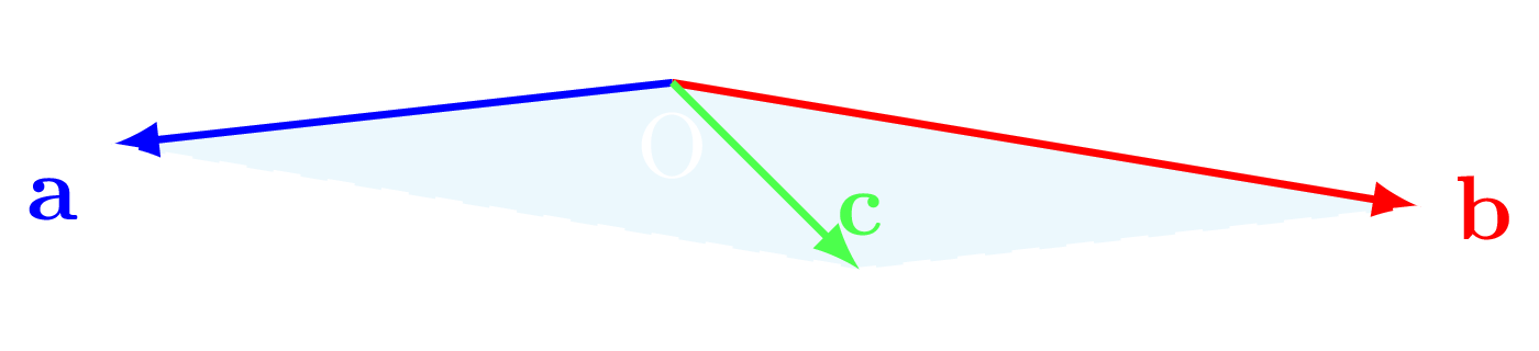
Suppose $\mathbf{a}, \mathbf{b}, \mathbf{c}$ are linearly dependent. Then one is a linear combination of the other two, say

\mathbf{c} = u\mathbf{a} + v\mathbf{b}.

If $\mathbf{a}$ and $\mathbf{b}$ are linearly dependent, then $O$ , $A$ , and $B$ are collinear, and $\mathbf{c}$ lies on the same line. Hence all four points are collinear, and therefore coplanar. If $\mathbf{a}$ and $\mathbf{b}$ are linearly independent, then the vectors of the form $r\mathbf{a} + s\mathbf{b}$ are exactly the points of the plane through $O$ spanned by $\mathbf{a}$ and $\mathbf{b}$ . Since $\mathbf{c}$ has this form, the point $C$ lies in that plane. Thus $O$ , $A$ , $B$ , and $C$ are coplanar.

Conversely, assume $O$ , $A$ , $B$ , and $C$ are coplanar. If $O$ , $A$ , and $B$ are collinear, then $\mathbf{a}$ and $\mathbf{b}$ are already linearly dependent, so the set $\{\mathbf{a}, \mathbf{b}, \mathbf{c}\}$ is dependent. If $O$ , $A$ , and $B$ are not collinear, then $O$ , $A$ , and $B$ determine a unique plane through the origin. Every point in that plane has position vector of the form $u\mathbf{a} + v\mathbf{b}$ . Since $C$ lies in this plane, its position vector satisfies

\mathbf{c} = u\mathbf{a} + v\mathbf{b}

for suitable scalars $u$ and $v$ . Geometrically, this may be seen by drawing through $C$ one line parallel to $\overrightarrow{OA}$ and another parallel to $\overrightarrow{OB}$ . These meet the lines generated by $\mathbf{a}$ and $\mathbf{b}$ at points $A'$ and $B'$ respectively, and then

\overrightarrow{OC} = \overrightarrow{OA'} + \overrightarrow{OB'}.

Since $A'$ lies on the line $OA$ , we have $\overrightarrow{OA'} = u\mathbf{a}$ ; since $B'$ lies on the line $OB$ , we have $\overrightarrow{OB'} = v\mathbf{b}$ . Hence $\mathbf{c}$ is a linear combination of $\mathbf{a}$ and $\mathbf{b}$ , so $\mathbf{a}, \mathbf{b}, \mathbf{c}$ are linearly dependent.

■

The figure below shows the coplanar situation $\mathbf{c} = \mathbf{a} + \mathbf{b}$ .

Three coplanar vectors a, b, and c in space with c equal to a plus b

We now negate the dependence criteria exactly as before.

Theorem 28 (Conditions for Linear Independence of Three Vectors)

Let $\mathbf{a}, \mathbf{b}, \mathbf{c} \in \mathbb{R}^3$ . The following statements are equivalent:

$\mathbf{a}, \mathbf{b}, \mathbf{c}$ are linearly independent.
The points $O, A, B, C$ are distinct and not coplanar (so they form a tetrahedron).
The equation $r\mathbf{a} + s\mathbf{b} + t\mathbf{c} = \mathbf{0}$ implies $r = 0$ , $s = 0$ , and $t = 0$ .

Proof

This theorem is obtained by negating the algebraic and geometric criteria proved above.

■

Remark (Determinant Preview)

For three vectors there is also a component criterion, analogous to the minor conditions for two vectors. Namely, $\mathbf{a}$ , $\mathbf{b}$ , and $\mathbf{c}$ are linearly dependent if and only if the determinant formed from their components is zero:

\det(\mathbf{a}, \mathbf{b}, \mathbf{c}) = a_1(b_2 c_3 - b_3 c_2) - a_2(b_1 c_3 - b_3 c_1) + a_3(b_1 c_2 - b_2 c_1) = 0.

While this is a necessary and sufficient condition, the rigorous development of determinant theory for $3 \times 3$ systems is reserved for the Linear Algebra notes. For the present chapter, the geometric and algebraic criteria established above are sufficient.

General Linear Independence and Dimension

We conclude our investigation of linear independence by formalising the relationship between a set of vectors and its subsets. These results, while simple, are used repeatedly and apply structurally to vector spaces of any dimension.

Theorem 29 (Inheritance of Dependence)

Let $\mathbf{a}, \mathbf{b}, \mathbf{c}$ be three vectors in $\mathbb{R}^3$ . If any one of them is the zero vector, or if any pair of them is linearly dependent, then the entire set $\{\mathbf{a}, \mathbf{b}, \mathbf{c}\}$ is linearly dependent.

Proof

If $\mathbf{a} = \mathbf{0}$ , then

1\mathbf{a} + 0\mathbf{b} + 0\mathbf{c} = \mathbf{0},

and the coefficients are not all zero. So the three vectors are linearly dependent. If a pair, say $\mathbf{a}$ and $\mathbf{b}$ , is linearly dependent, there exist scalars $r$ and $s$ , not both zero, such that

r\mathbf{a} + s\mathbf{b} = \mathbf{0}.

Then

r\mathbf{a} + s\mathbf{b} + 0\mathbf{c} = \mathbf{0},

again with coefficients not all zero. Hence the three vectors are linearly dependent.

■

Conversely, the property of linear independence is strictly inherited by subsets.

Theorem 30 (Inheritance of Independence)

Let $\{\mathbf{a}, \mathbf{b}, \mathbf{c}\}$ be a linearly independent set of vectors. Then they are distinct non-zero vectors, and any pair chosen from them is linearly independent.

Proof

This is the contrapositive of the preceding theorem. If one vector were zero, or if some pair were dependent, then the full set would be dependent. Therefore an independent triple must consist of distinct non-zero vectors, and every pair drawn from it must be independent.

■

The definition of dependence itself extends to any finite set.

Definition 26 (General Linear Dependence)

Let $n > 1$ be a natural number. A set of $n$ vectors is said to be linearly dependent if at least one of them can be written as a linear combination of the remaining $n-1$ vectors. If no such combination exists, they are linearly independent.

In $\mathbb{R}^3$ there is a strict upper bound on how many independent vectors can exist. The next theorem identifies that bound.

Theorem 31 (Dependence of Four Vectors)

Any four vectors $\mathbf{a}, \mathbf{b}, \mathbf{c}, \mathbf{d}$ in $\mathbb{R}^3$ are linearly dependent.

Proof

We seek scalars $r, s, t, u$ , not all zero, satisfying:

r\mathbf{a} + s\mathbf{b} + t\mathbf{c} + u\mathbf{d} = \mathbf{0}.

Substituting the explicit components $\mathbf{a} = \begin{bmatrix} a_1 \\ a_2 \\ a_3 \end{bmatrix}$ , $\mathbf{b} = \begin{bmatrix} b_1 \\ b_2 \\ b_3 \end{bmatrix}$ , etc., the vector equation translates into a system of three simultaneous linear equations:

\begin{cases} a_1 r + b_1 s + c_1 t + d_1 u = 0 \\ a_2 r + b_2 s + c_2 t + d_2 u = 0 \\ a_3 r + b_3 s + c_3 t + d_3 u = 0 \end{cases}

This is a system of three linear equations in four unknowns, and every equation has right-hand side zero. The algebraic fact recorded in the following remark states that such a system must have a solution other than

r = s = t = u = 0.

Thus there exist scalars $r, s, t, u$ , not all zero, satisfying the system, and therefore the four vectors are linearly dependent.

■

Remark (The Algebraic Step Used Above)

The proof uses the following fact: if one has fewer linear equations than unknowns, and every right-hand side is zero, then the system cannot force all unknowns to be zero. In the present case there are four unknowns but only three equations, so at least one parameter remains undetermined. Choosing that parameter to be non-zero produces a solution for which not all of $r,s,t,u$ vanish.

We leave the proof there, where it properly belongs: in the later discussion of Gaussian elimination, row reduction, homogeneous systems, pivots, free variables, and rank. In that setting we will prove the general statement that a homogeneous linear system with more unknowns than equations must admit a non-trivial solution.

It follows at once that any set of five or more vectors in $\mathbb{R}^3$ is also linearly dependent, since such a set contains a subset of four vectors.

This observation reveals a fundamental characteristic of the vector space. We have already seen that $\mathbf{e}_1$ , $\mathbf{e}_2$ , and $\mathbf{e}_3$ are linearly independent, but the theorem above shows that no fourth vector can be added to an independent set in $\mathbb{R}^3$ . The number $3$ is therefore the exact maximum.

Definition 27 (Dimension)

The dimension of a vector space is the maximum number of linearly independent vectors that can simultaneously exist within it.

The vector space $\mathbb{R}^3$ has dimension $3$ .
The vector space $\mathbb{R}^2$ has dimension $2$ .

This gives an exact algebraic meaning to the phrase three-dimensional space and aligns with the geometric intuition developed throughout the chapter.

Video

Lesson assets

Vectors and Geometry in Space

Cartesian Coordinates in Space

Orientation

The Bijection between Points and Triples

The Euclidean Metric in Space

The Equation of a Sphere

Vectors in Space

The Vector Space R3\mathbb{R}^3R3

Linear Combinations and Independence

Linear Independence of Two Vectors

Linear Independence of Three Vectors

General Linear Independence and Dimension

The Vector Space $\mathbb{R}^3$