
Solids, Planes, and Systems in Space
In Lesson 2AM we built the vector space , recovered the Euclidean metric through iterated Pythagoras, and worked out which collections of space vectors are linearly independent. What was still missing was any genuine use of that machinery against solid figures: tetrahedra, planes fixed by three non-aligned points, cevians viewed as segments inside a triangular slice of space. We now put the algebra to work. Each definition that follows is chosen so that the object it introduces earns its keep in the proof it enables, and each proof settles a question that space geometry had previously left open.
Displacement Vectors in Space
The first thing space geometry asks of us is a way to describe the relative position of two points without forcing the origin into every calculation. In Lesson 1PM we did exactly this in the plane by attaching the displacement to the directed segment . The construction transplants into component by component.
Let and be points in with position vectors and . The displacement vector associated with the directed segment is
In coordinates, if and , then
Because the algebraic laws of addition and scalar multiplication are identical in and , every theorem from Lesson 1PM whose proof used only those laws transfers without a single altered line. Three pieces will matter for the rest of this lesson:
- Midpoint Formula: the midpoint of has position vector .
- Collinearity: three points , , are collinear if and only if for some scalar .
- Parametric Line Equation: the line through distinct and consists of the points with , and the interpretation of fixed in Lesson 1PM is unchanged.
A triangle in space still lies in a unique plane, so any statement about a triangle proved purely from position vectors is inherited at once. In particular, the concurrency of medians at the centroid holds for a triangle placed anywhere in : the proof in Lesson 1PM never touched a second coordinate.
Let , , and . Then
The collinearity criterion is satisfied, so , , lie on a common line in space, and is in fact the midpoint of since the position vector of equals .
The Tetrahedron
With displacements and lines available, we can turn to a figure that cannot be drawn in the plane at all. A triangle is the smallest closed figure the plane admits; in space the smallest closed solid requires a fourth vertex lifted out of the plane of the first three.
A tetrahedron is the configuration determined by four points , , , in that are not coplanar. The points are its vertices; the four triangles , , , are its faces; the six segments , , , , , are its edges. Two edges are opposite when they share no vertex, and a vertex is opposite to a face when it is not one of the three vertices of that face.
The requirement that the four points not be coplanar is the spatial analogue of the non-collinearity demanded of the vertices of a triangle, and Lesson 2AM already supplies the exact test: the displacements , , must be linearly independent. Every tetrahedron therefore comes with a built-in certificate of its own three-dimensionality.
A triangle has three medians. A tetrahedron carries two families of distinguished internal segments.
Let be a tetrahedron.
- A median is the segment joining a vertex to the centroid of the opposite face.
- A bimedian is the segment joining the midpoints of two opposite edges.
There are four medians (one per vertex) and three bimedians (one per pair of opposite edges). Seven internal segments is a lot to keep track of, and the next theorem is precisely what keeps the picture tractable.
Let be a tetrahedron with position vectors . The three bimedians and the four medians are all distinct, yet they pass through a single common point
called the centroid of the tetrahedron. The centroid divides each median in the ratio , measured from the vertex towards the opposite face.
Consider first the bimedian joining the midpoint of edge to the midpoint of the opposite edge . By the midpoint formula,
The midpoint of the segment is therefore
The expression on the right treats symmetrically, so the argument by symmetry from Lesson 1PM forces to be the midpoint of the other two bimedians as well. All three bimedians therefore meet at .
Now fix the median from to the centroid of the opposite face . That face centroid is , and we can rewrite as
By the parametric line equation, lies on the segment at parameter , so divides in the ratio from vertex to face. Symmetry hands us the same conclusion for the medians issuing from , , and .
■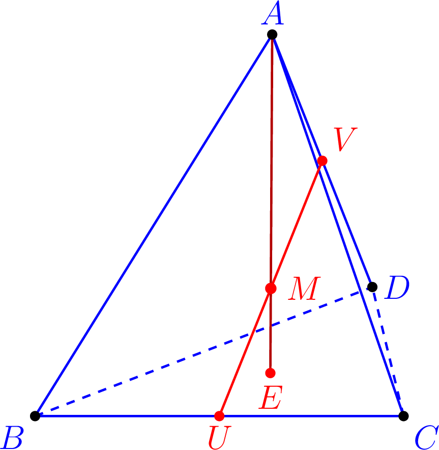
The figure above fixes the labels used in the proof: is the midpoint of , the midpoint of , and the centroid of face . The point is where the bimedian and the median intersect, and the same intersection holds for every other pair of median and bimedian by symmetry.
Let , , , . These four points form a tetrahedron because , , are linearly independent (each lies along a distinct coordinate axis). Its centroid is
The centroid of face is , and the identity confirms the division along the median .
Problem 20
The vertices of a tetrahedron are , , , . Compute the centroid, verify that the midpoint of the bimedian joining the midpoints of and coincides with it, and locate the point at which the median from meets the opposite face.
Planes, Barycentric Coordinates, and Ceva’s Theorem
The proof above quietly used a fact that deserves to be isolated: the average of three vertex vectors is the centroid of the triangular face they span, and more generally every point of that face is a weighted average of the three vertices. This is the geometric motivation behind the parametric equation of a plane, which plays the same structural role in as the parametric line equation did in .
The tetrahedron proof has already shown the first instance of this idea. When we wrote the centroid of face as
we were using a weighted average of the three vertices of that face. That is not a special trick reserved for centroids. More generally, every point in the plane determined by three non-collinear points can be described by weighting those three vertices, provided the weights add to . This is the planar analogue of the parametric line equation: on a line through and , the coefficients of and add to ; on a plane through , , and , the coefficients of , , and do the same.
Let , , be three non-collinear points in with position vectors . A point with position vector lies on the unique plane through , , if and only if there exist scalars , , satisfying
lies on precisely when is a linear combination of and , because , , are non-collinear and the two displacements are linearly independent. Expanding this condition,
and collecting terms gives
Setting yields the stated form with . The converse is immediate: such a combination rearranges back into , placing on .
■The triple is called the set of barycentric coordinates of relative to . Physically, they are exactly the weights one would place at , , so that the centre of mass of the weighted system sits at . When the centre of mass is the centroid, which recovers the formula we already used for the face centroid in the tetrahedron proof. This is not a coincidence: the tetrahedron centroid was constructed out of face centroids, and the face centroid is the simplest barycentric point.
Once points in a triangle are written in this weighted form, ratios along cevians become algebraic relations among the coefficients. With that perspective, the next theorem becomes almost purely algebraic, even though it is one of the oldest and most elegant results about triangles.
Let be a triangle, and let , , be points in the interiors of the sides , , respectively. Set
using the directed ratio from Lesson 1PM. The cevians , , are concurrent if and only if
Let be a point in the plane of , written in barycentric form as
Since , the directed-ratio formula from Lesson 1PM gives
Thus lies on the cevian if and only if
for some scalar . Substituting the expression for shows that the coefficients of and in such a point satisfy
In the same way,
Suppose the three cevians meet at a common point. Then the barycentric weights of that point satisfy all three ratio conditions simultaneously, so
Conversely, assume . Because , , lie on the sides of the triangle, the directed ratios , , are positive. Define
This is a genuine point of the plane because the denominator is positive. Its barycentric coordinates are proportional to , so
where the last equality uses . Each ratio places on the corresponding cevian, so , , meet at .
■This is the affine version of Ceva’s theorem for points chosen on the actual sides of the triangle. If one allows , , to range over the full lines determined by those sides, then the condition also includes an exceptional case in which the three cevians are parallel. We do not pursue that extension here.
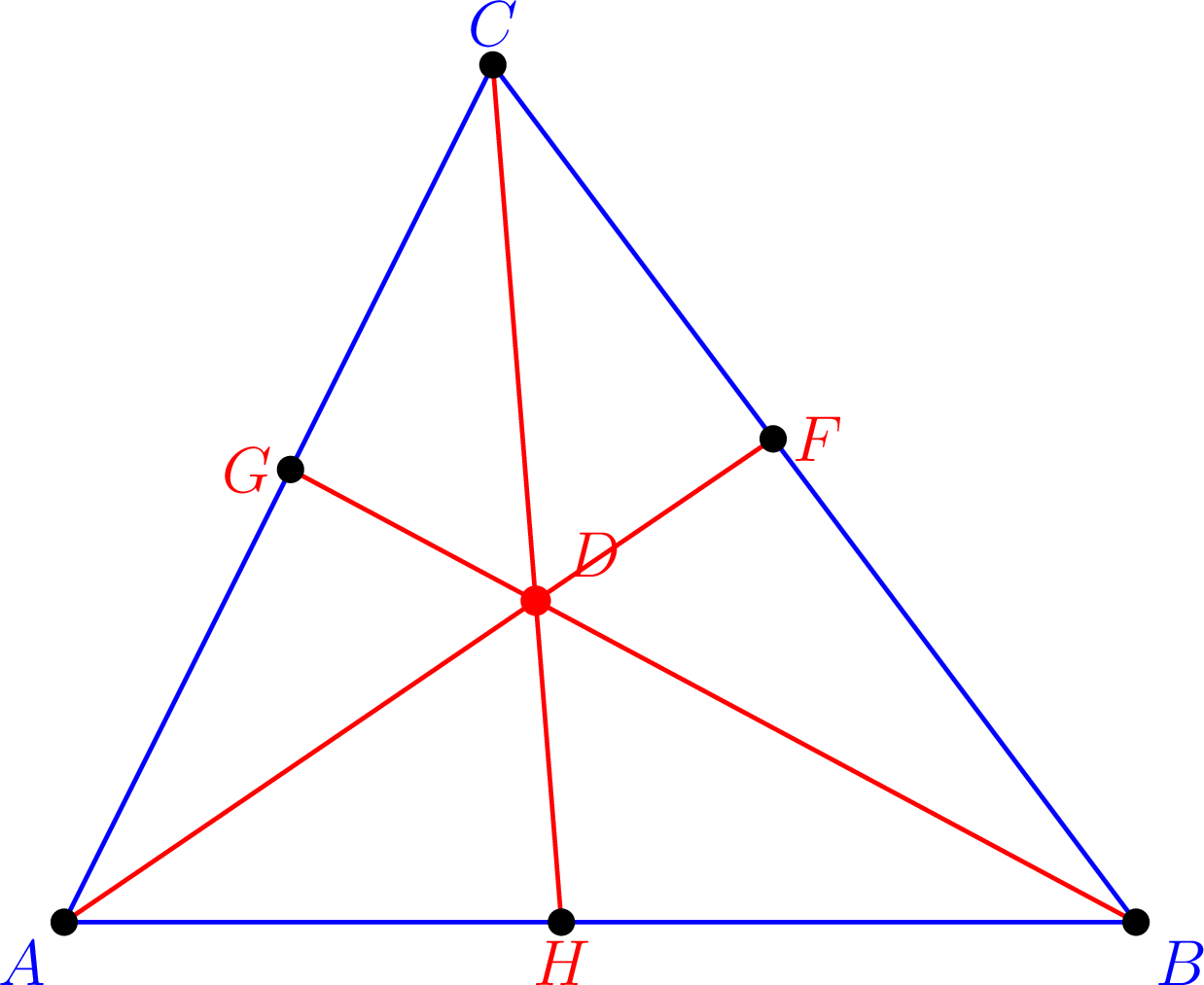
Setting forces , , to be the midpoints of their respective sides, turning the cevians into medians. Since , Ceva’s theorem instantly reproduces the concurrency of medians proved in Lesson 1PM. The centroid is not an isolated coincidence, but the simplest worked example of a general principle about cevians.
In a triangle , place on with and on with . For the three cevians , , to pass through a common point, Ceva’s theorem demands
Equivalently, divides so that , i.e. sits one seventh of the way from to . Any other placement of produces cevians that fail to share a single intersection.
Problem 21
In a triangle , let be the midpoint of and let divide with . Determine the location of on line for which the cevians , , are concurrent, and state the result using the directed ratio convention from Lesson 1PM.
The Dot Product in Space
Everything to this point has been affine: positions, displacements, ratios along lines, concurrence. To say anything about lengths and angles inside a spatial figure, we need the dot product again, and we need it for three-component vectors. The extension is dictated by the component structure set up in Lesson 2AM.
Let and be vectors in . Their dot product is the real number
The only change from Lesson 1PM is the presence of a third summand. As in the planar case, the self dot product recovers the square of the magnitude fixed in Lesson 2AM:
so the Euclidean distance between space points can be written as , bridging the dot product and the distance formula from Lesson 2AM.
For all and all :
- Symmetry: .
- Bilinearity: , and symmetrically in the second argument.
- Positive Definiteness: , with equality if and only if .
The component-wise verification from Lesson 1PM gains only one extra term per identity when the vectors carry three components instead of two, and each identity is preserved under that addition. No new argument is required.
■Metric Identities in Space
Because the algebraic laws of the dot product are the same in and , the entire chain of metric inequalities already proved in Lesson 1PM rebroadcasts into space with no further work.
Let and . Then:
- Homogeneity: .
- Parallelogram Law: .
- Cauchy-Schwarz Inequality: .
- Triangle Inequality: .
- Law of Cosines: .
Each item was proved in Lesson 1PM using nothing beyond symmetry, bilinearity, and positive definiteness of the dot product, together with the identity . All three ingredients hold in by the preceding theorem, so the planar proofs apply verbatim.
■The absence of any new work here is itself the punchline. Metric geometry in space inherits metric geometry in the plane once the algebraic framework is in place; and the reason is simple enough to state precisely. Any triangle drawn inside a spatial figure lies in a plane of its own, and every metric inequality above is a statement about pairs of vectors that collectively span at most a single plane.
Angles, Orthogonality, and Projection
Because the Cauchy-Schwarz inequality still holds, the quantity remains in for all non-zero . The definition of angle used in Lesson 1PM lifts to space without modification.
For non-zero , the angle between them is the unique number satisfying
Two space vectors are orthogonal, written , when , which agrees with the planar convention from Lesson 1PM.
This is consistent with the geometric angle formed by the segments and : the triangle lies in the unique plane determined by and , and inside that plane the angle reduces to the planar one. The ambient third dimension plays no role.
Let
Then
Hence the angle between them satisfies
so
The negative cosine confirms that the angle is obtuse.
Return to the tetrahedron with , , , . The edges and meet at vertex , and the angle between them satisfies
so . A parallel computation shows that and , so the three edges meeting at form a right-angled corner, which is exactly the expected behaviour once each edge is placed along a distinct coordinate axis.
Consider the unit cube in with vertices satisfying . Take the diagonal from
and the diagonal from
The corresponding displacement vectors are
Hence
So
This gives the obtuse angle between the chosen directed diagonals. The acute angle between the two diagonal lines is therefore
Problem 22
Find two non-zero vectors perpendicular to
that are not scalar multiples of each other. Then find one unit vector perpendicular to this vector, and describe geometrically the full set of all vectors perpendicular to it.
The dot product machinery already gives a clean proof of the Law of Sines. Take a triangle and direct its three sides cyclically by vectors , , , so that
At the vertex where the sides and meet, let the interior angle be , and let the opposite side have length . By the angle formula,
so
Now use . A direct expansion shows
Hence
The right-hand side is unchanged by permuting , , , so the same value is obtained from each of the three vertices of the triangle. Since each interior angle lies in , its sine is positive, and therefore the ratio itself is the same at all three vertices. That is exactly the Law of Sines.
Orthogonal Projection
Resolving a vector into a component along a reference direction and a component perpendicular to it is another theorem that needs no new proof: the argument in Lesson 1PM depended only on bilinearity and positive definiteness. In space, the decomposition still takes place inside a plane, namely the plane spanned by the two vectors involved.
Let be a non-zero vector. For every there is a unique decomposition
in which the scalar is
The vector is called the orthogonal projection of onto .
Write and impose . This yields . Since , positive definiteness gives , so is forced to equal . With fixed, the vector is determined, and uniqueness of the decomposition follows.
■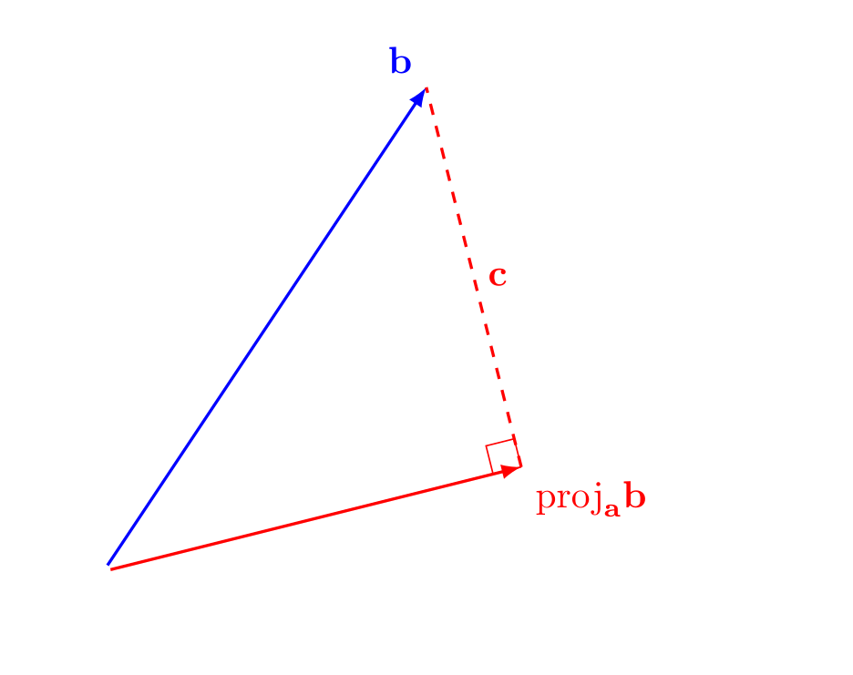
The triangle with vertices , , lies in the plane spanned by and and is right-angled at the tip of the projection. Its hypotenuse has length and the leg along has length
Reading the inequality hypotenuse leg out of this triangle gives a purely geometric proof of Cauchy-Schwarz, this time without a discriminant in sight. The equality cases of the metric inequalities now fall out immediately.
Let .
- if and only if and are linearly dependent.
- if and only if one of the vectors is a non-negative scalar multiple of the other.
For (i), if and are dependent then either one of them is the zero vector, in which case both sides are zero, or for some scalar , in which case both sides equal .
Conversely, suppose
If or then the vectors are trivially dependent, so assume both are non-zero. By the projection theorem,
Then
so the equality hypothesis gives
Squaring,
But orthogonality gives
so . Hence and therefore , proving dependence.
For (ii), square the supposed equality to obtain
which reduces to . This is simultaneously the Cauchy-Schwarz equality (hence dependence, by (i)) and the statement that is non-negative, which for dependent vectors means one is a non-negative multiple of the other.
■Let and . Then and , so
The orthogonal component is
and the check confirms that the decomposition is correct.
Problem 23
Let and . Compute the angle between and , the orthogonal projection of onto , and the length of the resulting orthogonal component. Verify directly that the component you produce is perpendicular to .
Planes in Space
The orthogonal projection just developed turns the dot product from an angle-measuring device into a way of writing down loci. A plane in is the simplest such locus: fix a direction, and demand that every displacement from a chosen point be orthogonal to it. Unpacking that single sentence delivers the whole elementary theory of the plane as a set of points, and its results will recover in space everything Lesson 1PM established for the line in the plane.
Begin with the homogeneous linear equation
which the dot product collapses to , where
This is the set of position vectors orthogonal to the fixed vector , which is precisely the plane through the origin with as its normal. A general plane need not pass through the origin, but the inhomogeneous form
handles that case with no structural change. If is any point on the plane, with position vector , then , so , and substituting back rewrites the defining equation as
Read geometrically, the plane is the set of points whose displacement is orthogonal to . Every choice of produces the same locus; only the algebraic label shifts.
A linear equation
with defines a plane in , and the vector
is a normal vector to that plane.
Problem 24
Let
Find a non-zero vector perpendicular to . Then show that the vectors perpendicular to are exactly those whose coordinates satisfy
Finally, find a non-zero vector perpendicular to the plane
A plane that meets the coordinate axes at , , and , with , , all non-zero, is described by the compact equation
Each intercept satisfies this by inspection: at , the left-hand side is , and the other two are analogous. Clearing denominators,
so by the previous theorem the vector
is a normal to the plane.
Distance from a Point to a Plane
The point-line distance problem in the plane was solved in Lesson 1PM by projecting a displacement onto the normal of the line. The same strategy works in space, and this is the first place the orthogonal projection theorem earns its keep against a problem with no honest two-dimensional version.
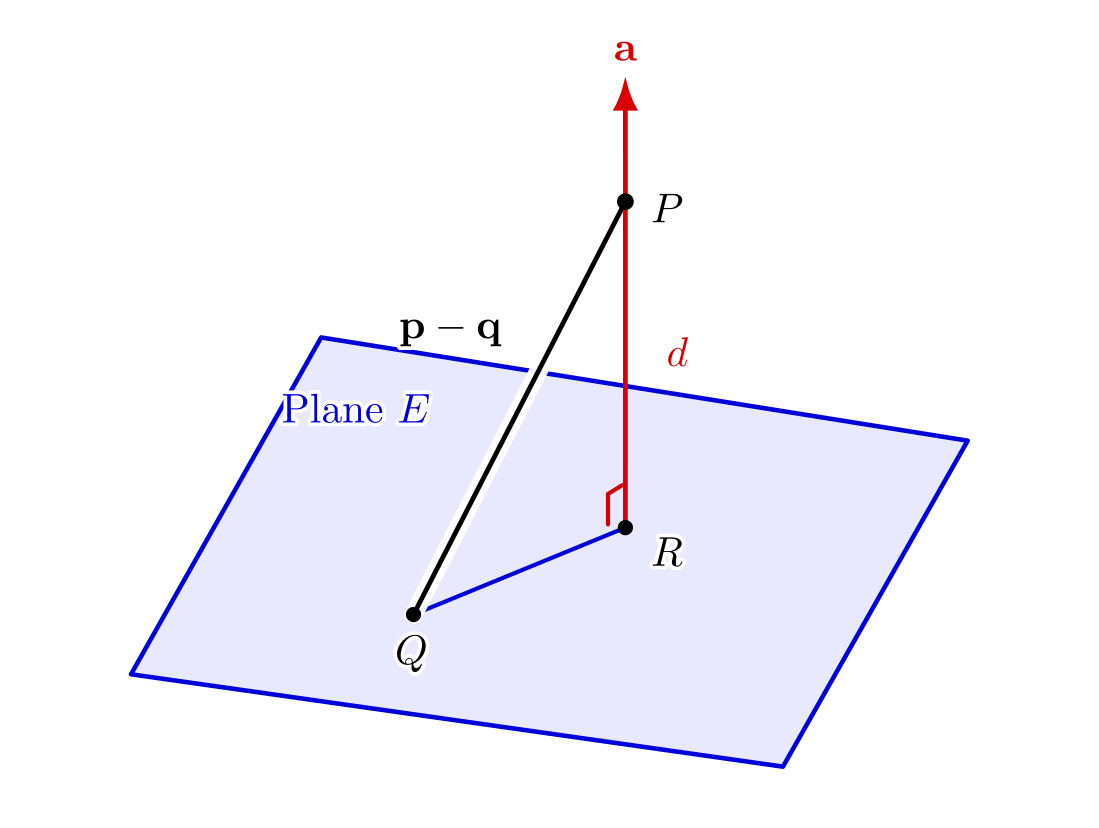
Let be the plane defined by , where , and let be a point with position vector . The perpendicular distance from to is
Let be any point on and let be the foot of the perpendicular from to . The displacement is parallel to , since both are orthogonal to every direction inside the plane, so is exactly the orthogonal projection of onto :
Taking magnitudes,
Since lies on , , and the stated formula follows.
■
Dividing the defining equation through by recasts the plane into its normal form
and in this form the distance formula collapses to , where denotes the linear polynomial on the left. The value of at any point is literally its signed distance from the plane, which is a small but extremely useful fact: wherever we have a plane written in normal form, the function doubles as a ruler.
Let define a plane , and let , be points on opposite sides of so that the segment meets at a unique point . The position of on the segment, recorded through the directed ratio from Lesson 1PM, is
To see this, observe that divides in the ratio , so
The condition combined with the linearity of the dot product gives
from which is immediate. The signed values of at the endpoints therefore encode the division ratio directly, and this observation is the bridge we will need for sheaves of planes below.
Problem 25
Let be the plane
(a) Find the distance from the point to .
(b) Rewrite the equation of in normal form
with .
(c) Use the normal form to determine the signed distance of from .
Systems of Planes
A single plane is one linear condition. Two or more planes turn solid geometry into linear algebra in miniature: whether they meet, how they meet, and which further planes are generated by their intersection. The remainder of the lesson treats these questions with the tools already in hand.
Parallel Planes
Write two planes and as
with respective normals and . The planes are parallel precisely when their normals are collinear, i.e. for some non-zero scalar . Dividing the equation for through by replaces its normal by without altering the locus, so no information is lost by assuming from the outset that two parallel planes are presented with a common normal vector.
The distance between two parallel planes and is
Pick any point on . Then , so . The Distance to a Plane theorem applied to and gives
Because was arbitrary and every point of is the same perpendicular distance from , this common value is .
■Problem 26
Find the distance between the parallel planes
and
First rewrite them with a common normal vector, and then apply the parallel-plane distance formula.
Intersecting Planes and Sheaves
Two planes that are not parallel share an entire line. Their normals and are linearly independent and together span the plane orthogonal to the intersection line , while the direction of itself is the unique space direction (up to sign) orthogonal to both. The natural numerical quantity attached to such a pair is the angle between them, defined through their normals:
The absolute value pins the result to the dihedral angle along , ignoring the irrelevant orientation of the two normals.
The more interesting question is algebraic: which linear equations describe the remaining planes that contain ? The answer is remarkably clean, and hinges on the observation that any linear combination of and still vanishes on .
Let and be two distinct planes meeting in a line . The sheaf (or pencil) of planes through is the set of all planes in that contain .
Let and define two distinct planes meeting in the line . A plane belongs to the sheaf through if and only if it can be written as
for some pair of scalars .
Suppose first that is given by for some . Every point of satisfies and simultaneously, hence it also satisfies the combined equation, so and lies in the sheaf.
Conversely, let be an arbitrary plane through , with normal and constant term . The vector is orthogonal to the direction of , so it lies in the two-dimensional subspace spanned by and ; there are therefore scalars and with . The linear form has leading part and vanishes on every point of , while also vanishes on by construction. Two linear forms with the same leading part that agree on any single point are identical, so , and has the stated form.
■The sheaf equation is, at bottom, the observation that containing is itself a linear condition on the space of linear equations. Its real utility is that it converts statements about the geometry of the sheaf into statements about pairs , and in doing so exposes an invariant that is not at all apparent from the geometry alone. For that invariant we need one more classical notion, which is new to this course but built entirely out of quantities we have already met.
Let be four distinct collinear points. Their cross-ratio is the quotient of directed ratios
where is the directed ratio along the common line from Lesson 1PM.
Let be four distinct planes in a common sheaf with common line , and let be a transversal line that meets each in a unique point , does not lie in any of the four planes, and does not meet . The cross-ratio depends only on the four planes, not on the transversal line .
Pick two planes of the sheaf defined by linear forms and , with the extra choice that the plane is not one of . This is possible because the sheaf contains infinitely many planes. Then every can be written in the affine chart
for finite scalars . Let meet the four planes at with position vectors . Since does not meet , none of the points lies on the auxiliary plane , so the values are all non-zero.
The plane is defined by the linear polynomial , and the Ratio of Division computation from the previous section, applied along the transversal line , yields
Since lies on we have , so , and similarly . Substituting and cancelling the common factor of in numerator and denominator,
The same calculation with replaced by gives the directed ratio in which divides . Forming the cross-ratio as the quotient of these two directed ratios, the prefactor (which is the only place the transversal enters the formula) cancels, leaving
The right-hand side is built entirely from the parameters of the four planes in the sheaf and contains no trace of , so the cross-ratio is independent of the transversal.
■Problem 27
Suppose four planes in a common sheaf are written in the affine chart
(a) Compute the cross-ratio
on any transversal line meeting the four planes.
(b) Explain why your answer is independent of the chosen transversal.