
More on Planes and Systems
Lesson 2PM attached every plane in to a single linear expression and identified its normal vector. That description is enough for asking whether a given point lies on the plane, but several natural questions involve the plane only incidentally. A computer rendering a scene has to decide, for every pair of objects, whether a flat surface between them blocks the line of sight; a parametric animation of a ball rolling along a tilted roof has to stay on the surface at every frame. Neither question is answered by finding a point of the plane. The first needs an algebraic test for which side of the plane a point lies on, and the second needs a description that produces points of the plane rather than one that checks them. Both live a short algebraic step from the material we already have, and this lesson walks the step.
Parametric Description of a Plane
The Parametric Equation of a Plane from Lesson 2PM wrote every point of the plane through three non-collinear points , , as a barycentric combination with . Using the constraint to eliminate rearranges that combination into
with base point and direction vectors , lying inside the plane. The three-point form and this “base point plus two directions” form carry the same information, but the latter is the natural input whenever the plane comes to us through a point on it together with two independent directions it contains, rather than through three named vertices.
Let and let be linearly independent. The set
is a plane in , and every plane arises from some such triple . Each point of corresponds to a unique pair .
The three position vectors , , correspond to non-collinear points because and are linearly independent, so the Parametric Equation of a Plane from Lesson 2PM identifies with the unique plane through them. If then , and linear independence forces , , proving uniqueness of the parameters.
Conversely, let be an arbitrary plane and pick three non-collinear points with position vectors . The displacements and are linearly independent, and the Parametric Equation of a Plane writes every point of in the required form with .
■The pair is a coordinate system inside the plane, with axes pointing along and . These internal axes need not be perpendicular, and when the plane is viewed from a steep angle the induced grid can look distorted, in the same way that a tilted surface appears foreshortened from the side.
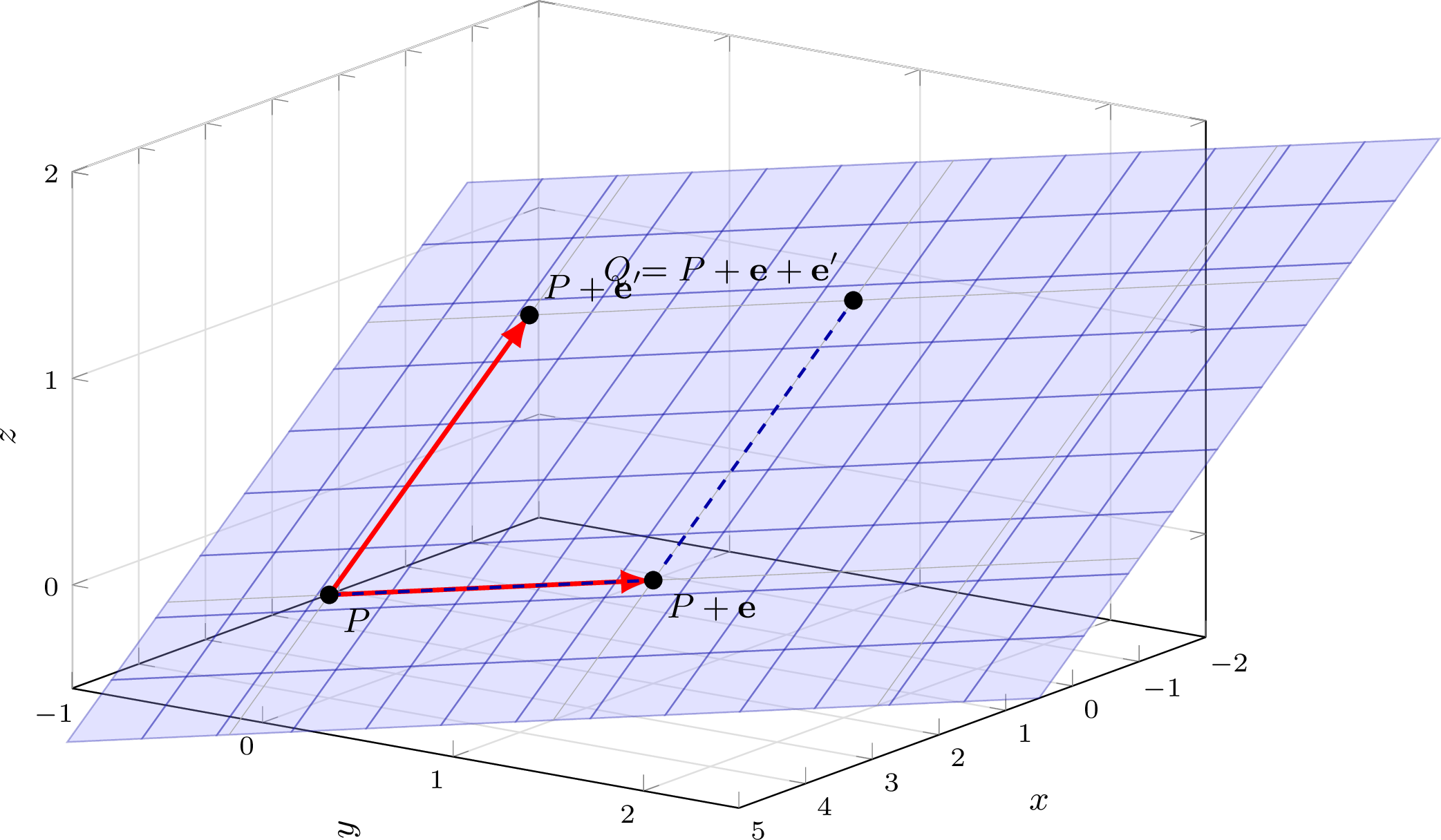
The figure above realises the example from the next subsection: the base point is , the direction arrows are and , and the sample point is reached by the dashed parameter route . In the internal -coordinates of the plane, sits at .
Translating Between Forms
The equational form and the parametric form answer different questions, and most practical work with planes involves passing from one to the other. The mechanical content of each conversion is short enough to absorb through a worked example.
Parametrise the plane .
Solve for one coordinate in terms of the others: . Taking and as free parameters,
which places the plane in parametric form with base point and direction vectors
These directions must be orthogonal to the normal
and indeed and , as required.
Find an equation for the plane through , , .
The displacements
span the directions inside the plane, so a normal vector
is determined by the two orthogonality conditions
The first gives and the second , so up to scale
The constant is pinned down by demanding that satisfy the equation: letting denote the position vector of ,
The resulting plane coincides with the one parametrised in the previous example, as intended.
The construction tacitly assumes that are non-collinear, and that hypothesis is easiest to check directly on the displacement vectors: three points lie on a common line precisely when one of is a scalar multiple of the other, with a positive multiple putting and on the same side of and a negative multiple putting them on opposite sides. Otherwise the two displacements span a genuine plane through , and the procedure of the previous example goes through.
For , , ,
An equation would force in the first coordinate, which has no solution, so the two displacements are not scalar multiples of each other. The three points are therefore non-collinear and determine a plane; running the recipe of the previous example on them gives normal and equation .
Starting from a Point and a Normal
A third natural input packages a plane as a point lying on it together with a vector perpendicular to it. The equational form is immediate from the perpendicularity of to every displacement inside the plane:
Passing to a parametric form requires two linearly independent directions orthogonal to . A reliable recipe, which sidesteps the cross product and so generalises verbatim to , is to read off two auxiliary points of the plane by fixing two of the three coordinates at convenient values (typically and ) and solving the equation for the third. Repeating with a different coordinate held constant gives a second auxiliary point, and a quick collinearity check on the two displacements from certifies that they are independent.
Give equational and parametric descriptions of the plane through with normal .
The perpendicularity condition expands to
For the parametric form, set : gives , so lies on the plane. Set : gives , so lies on the plane. The displacements
disagree in first coordinate ( versus ), so they are not scalar multiples, and
parametrises the plane.
When the plane instead passes through the origin, the recipe shortens, because supplies the base point and forces the constant term to vanish. For the plane through with normal , the equation is ; setting gives , and setting gives . The displacements from are and themselves, not scalar multiples (their -coordinates are and ), and
parametrises the plane.
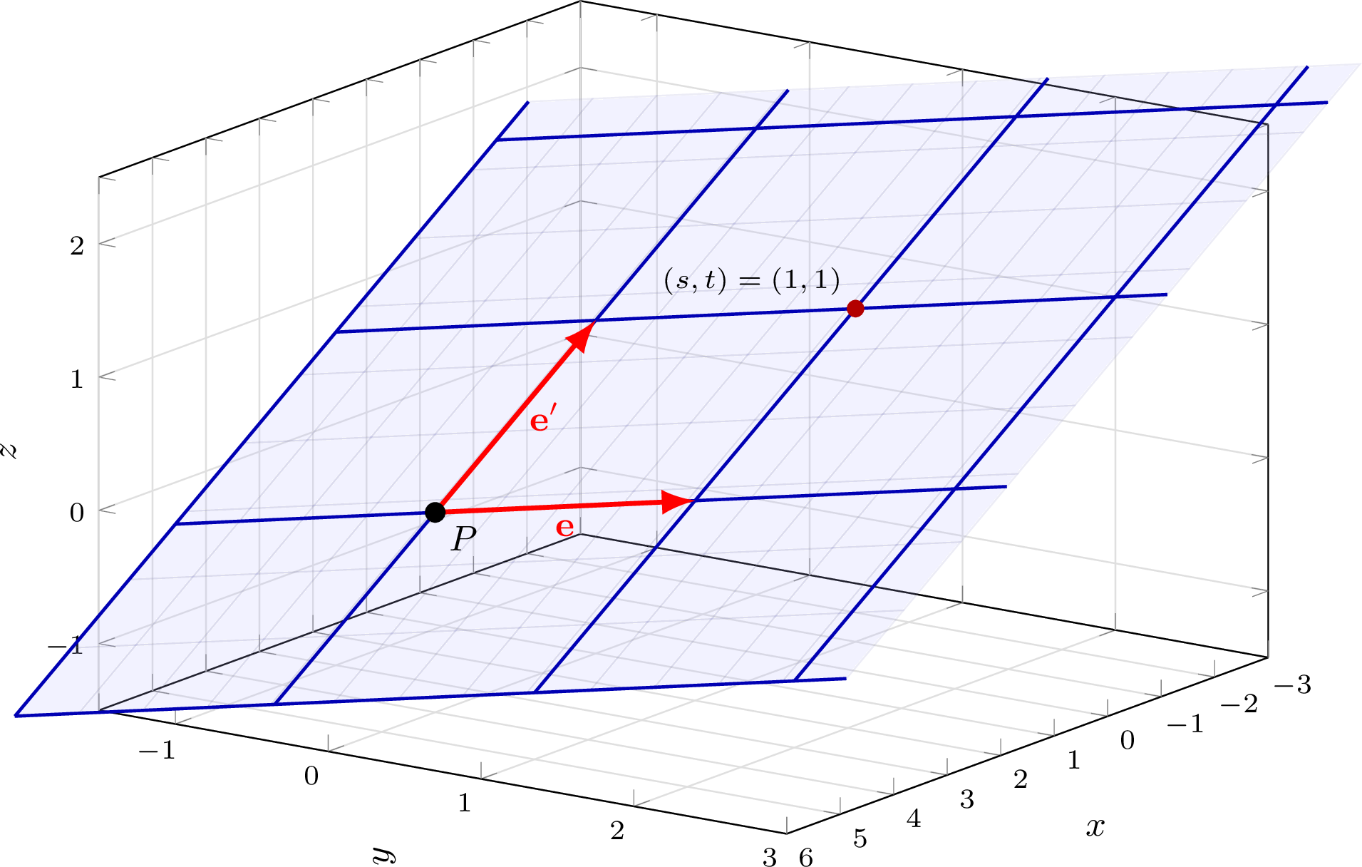
The lattice in the figure is the image of the integer -grid under the parametrisation of the plane from Example 41. The two families of gridlines are the fibres and , each itself a line inside the plane, and they meet at the lattice points.
Traces Inside a Plane
One payoff of the parametric form is that it constrains motion to the plane for free. For any continuous curve in the -parameter space, the composition
is automatically a continuous curve in lying entirely on the plane. The equational form offers no such guarantee, so whenever the task is to generate points on a plane, for example when rendering a path along a surface, the parametric form is the right tool, whereas whenever the task is to test points already in hand, the equational form is.
Sides of a Plane
A plane partitions into three disjoint pieces: the plane itself and the two open regions on either side. The linear expression whose zero set defines the plane already contains the information needed to tell these regions apart: the only thing that changes between them is the sign of that expression.
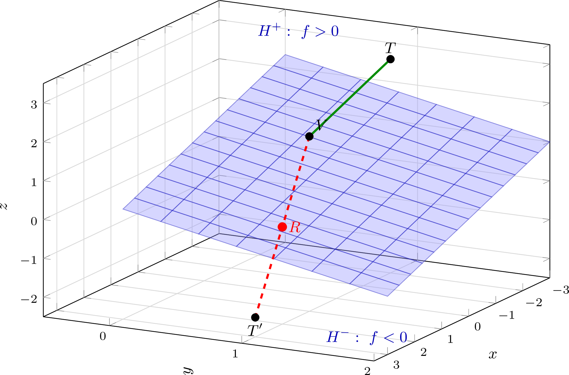
Let with , and let be the associated plane. The open half-spaces of are
Two points lie on the same side of when and share a sign, and on opposite sides when the signs differ.
Every point of belongs to exactly one of , , , since takes a unique real value at each point and the three cases , , exhaust the possibilities. The geometric question of which side of a point lies on therefore reduces to a single sign comparison, and the algebraic shortcut extends to the related question of when two points are separated by the plane.
Let define a plane , and let be points with . The segment meets if and only if and have opposite signs, and in that case the intersection point is unique.
The Ratio of Division by a Plane from Lesson 2PM fixes the location of the intersection of the line with : a point with directed ratio lies on precisely when
Because , the denominator is non-zero, so is a well-defined real number. The intersection lies on the closed segment rather than on its extension exactly when , and this inequality holds if and only if and have opposite signs (the case corresponds to , which the hypothesis excludes). Uniqueness of gives uniqueness of .
■The test turns the geometric question of whether a plane separates two points into one arithmetic evaluation per point. That is the mechanism behind one of the basic primitives in three-dimensional rendering, and it also sits at the algebraic heart of a much larger family of questions across dimensions.
A video game places a viewer at at the bottom of a driveway, and a tree at in the backyard. The relevant section of roof lies in the plane . Does the roof block the viewer’s sight of the tree?
Set and evaluate:
Both values are positive, so ; by the Sign Test the segment does not meet and the sight line is unobstructed. If the tree were instead at , the evaluation would give , placing . The signs at and would then disagree, the segment would cross , and the Ratio of Division by a Plane would place the obstruction at directed ratio
i.e. at the midpoint of the sight line.
The entire discussion above uses only the sign of a single linear expression and so transplants verbatim to : a linear form on cuts space into a hyperplane and two open half-spaces, and the same sign test decides when a segment between two points is split by the hyperplane. In large this is exactly the linear-algebraic machinery behind separating hyperplanes in convex optimisation and support vector machines, but the proof ingredients are the ones already used in .
Problem 28
Let be the plane , and let , , . Determine which pairs among lie on the same side of and which lie on opposite sides. For each separated pair, use the Ratio of Division by a Plane from Lesson 2PM to compute the directed ratio at which the connecting segment meets .
Lines in Three-Dimensional Space
A line in is not the zero set of a single linear expression, since that zero set cuts out a plane. The parametric form, which carried two direction vectors alongside a base point when describing a plane, collapses to the natural description of a line once a single direction is kept.
Let and let be non-zero. The set
is the unique line through with direction , and each point of corresponds to a unique . Every line in arises from some such pair .
When the line is presented through two distinct points , the displacement supplies the direction, and the parametric form becomes
which recovers at , at , and the midpoint of at . For , the Directed Ratio from Lesson 2PM is
so the parameter determines the directed ratio, but is not itself the directed ratio.
For base point and direction , the line through along is
For the line through the distinct points and , the direction is , and
The single-parameter description of a line and the two-parameter description of a plane are algebraic shadows of their geometric dimensions, and the number of free parameters needed to sweep out a figure will be our first handle on the notion of dimension in later lessons, where it extends far beyond the of daily experience.
Assembling a Plane from Parallel Slices
Throughout this lesson and the last, every equation with has been treated as the zero set of a plane, without a derivation of that fact from anything more primitive. One way to see why the claim is true is to assemble the surface from its slices by vertical planes, building on the familiar fact that a linear equation in two variables cuts out a line.
Relabelling axes if necessary, arrange that and divide through to put the equation in the form
Fixing collapses the equation to , a line of slope in the -plane sitting at , with vertical intercept . As varies, these parallel-sloped lines stack to form the full surface, and the intercept is linear in , so its graph is a straight ruling and the stacked slices fit together flat.
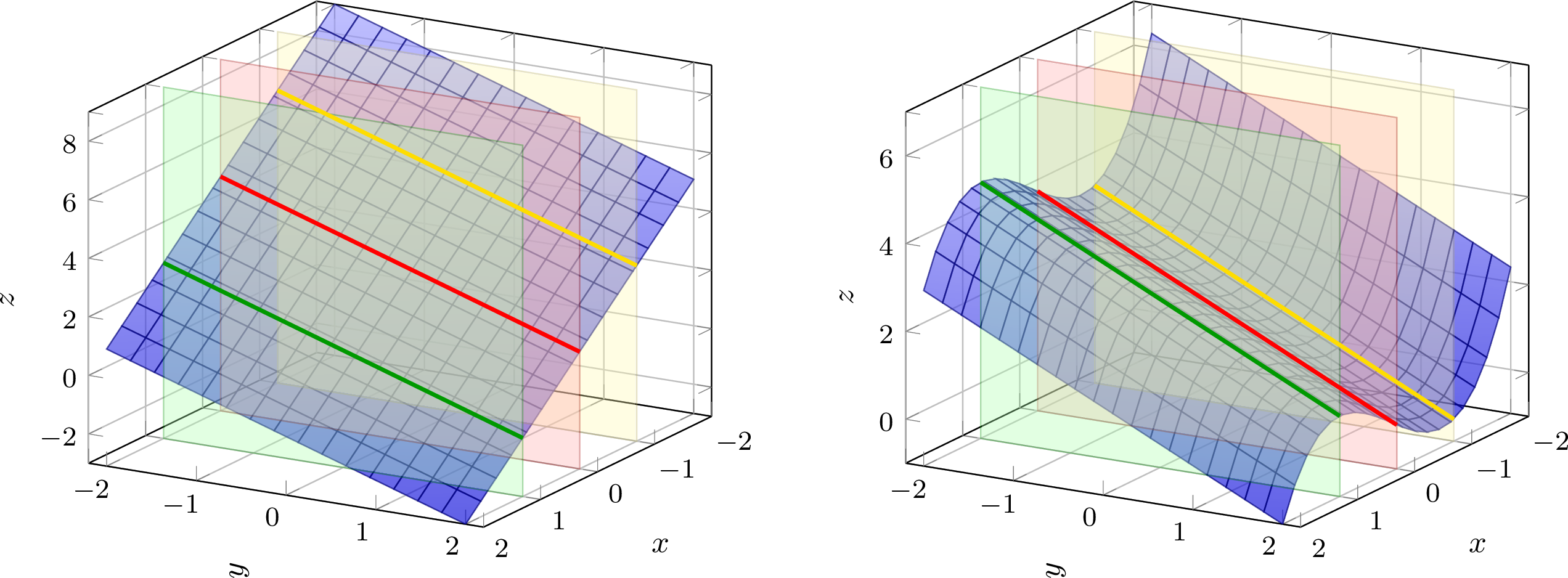
The contrast with the right-hand surface is instructive. Both pictures show a surface whose every slice is a line of slope in the -plane. On the left the intercept depends linearly on and the stacked slices produce the plane ; on the right is a cubic, and the same parallel-slope lines assemble instead into a wavy ruled surface. Linearity of in is the structural ingredient that turns a family of parallel slices into a flat plane, and its absence is what allows an assembly of parallel-slope lines to buckle.
Problem 29
Let be the line through with direction , and let be the plane . Find the value of at which the parametrisation meets , give the coordinates of the intersection point, and determine whether that intersection lies between and on the line or outside the segment.
Toward Systems of Linear Equations
Every equation encountered in this lesson is a single linear equation in three unknowns, cutting out a plane in . Problem 29 already nudged past that one-equation setting: finding where a line meets a plane is the problem of jointly satisfying the line’s three parametric equations and the plane’s single equation, four scalar constraints tying together four unknowns . The intersection of two non-parallel planes is the joint solution set of their two defining equations in three unknowns, and the intersection of three generic planes is the joint solution set of three. Each configuration is a small instance of one general object: a system of linear equations.
The general system of linear equations in unknowns has the form
with coefficients and right-hand sides . Equivalently, the th equation may be written in the compact summation form
When every the system is called homogeneous, and otherwise inhomogeneous. Both the and the are drawn from a chosen field, and we write for such a generic field: a set carrying addition, subtraction, multiplication, and division subject to the nine field axioms (A1)-(A9) laid out for the real numbers in the MCEA lesson “Predicates, Numbers, and Sets”. Those nine axioms, and only those, are what every manipulation in the chapters ahead is ultimately allowed to invoke, so any statement proved from them applies uniformly to every choice of ; the familiar ones are , , and , and unless stated otherwise will mean one of these three with the default reading .
Systems of this form have been studied since the beginnings of algebra in its modern sense. Newton’s Arithmetica Universalis, compiled from his Cambridge lectures of the 1670s and published in 1707, already set out systematic elimination for small linear systems; and the matrix notation that packages the coefficients into a rectangular array was introduced by Arthur Cayley in his 1858 Memoir on the Theory of Matrices, building on the determinantal calculus developed a few years earlier by his Cambridge colleague James Joseph Sylvester. The linear-algebraic investigation of such systems has since grown into the hub of the whole subject, dragging along with it the theories of linear spaces, linear transformations, and matrices.
Three basic questions organise everything that follows.
- Existence. Does the system have any solution at all?
- Uniqueness. When a solution exists, is it the only one?
- Structure. When there are infinitely many solutions, what geometric shape does the solution set have, and how is it parametrised?
For the tiny cases visited in this lesson and the last, geometry in and already answers all three at a glance: two non-parallel lines in the plane meet in a single point; two non-parallel planes in meet in a line, a one-parameter family of solutions; three generic planes in meet in a point; and two parallel but distinct planes meet in the empty set. In higher dimensions, and with more than three equations, that intuition runs out, and we will need a systematic algebraic procedure together with the language of matrices and ranks to reduce existence, uniqueness, and structure to bookkeeping. That procedure, and the vocabulary that goes with it, is the subject of the next few lessons, where we work out row reduction for arbitrary systems and see how it settles all three questions uniformly.
Problem 30
Consider the system
How many equations and unknowns does it have? Is it homogeneous or inhomogeneous? What geometric object does each equation define in , and what shape should you expect for the full solution set before carrying out any elimination?