18/03/2026

#Math#Differentiation

Video

Lesson assets

video link

CS50P Lecture 0: Functions, Variables

recitation

Recitation

Homework 6 PDF

Newton’s Method

In Lesson 6AM we solved every “find $r$ from $e^{r T} = M/P$ ” question by taking $\ln$ of both sides, so each unknown reduced cleanly to a closed-form expression in $\ln$ . The Picasso problem solved $e^{56 r} = 6914.29$ ; the doubling-time problem solved $e^{0.05 t} = 2$ ; the matching-rate problem solved $e^{r^{\ast}} = (1 + 0.05/12)^{12}$ . Every equation in that lesson admitted an exact closed-form answer because the operations involved were already invertible in the toolkit we’d built up by Lesson 5PM.

Most equations we meet in practice are not so kind. The bookkeeping equation

x \, e^{x} = 1, \tag{1}

which arises whenever the half-life of one process must equal the time constant of another, has no solution expressible using the functions in our current toolkit: $+, -, \times, \div$ , roots, $\ln$ , and $e^{(\cdot)}$ . The polynomial equation

x^{4} + 2 x^{3} - x^{2} - 1 = 0, \tag{2}

which arises in a structural-engineering load problem, does admit an exact root formula (the quartic formula), but the formula is too unwieldy for routine work. The single positive solution is approximately $x \approx 0.8445$ , and the closed form is several lines of nested radicals.

Both equations have the same shape: $f(x) = 0$ for an explicit, differentiable $f$ . Our closing application of MA0A turns the entire derivative toolkit toward a numerical method that produces such $x$ to as many decimals as desired, using only $f$ and $f'$ . The key is the linear approximation that the derivative supplies us at each point.

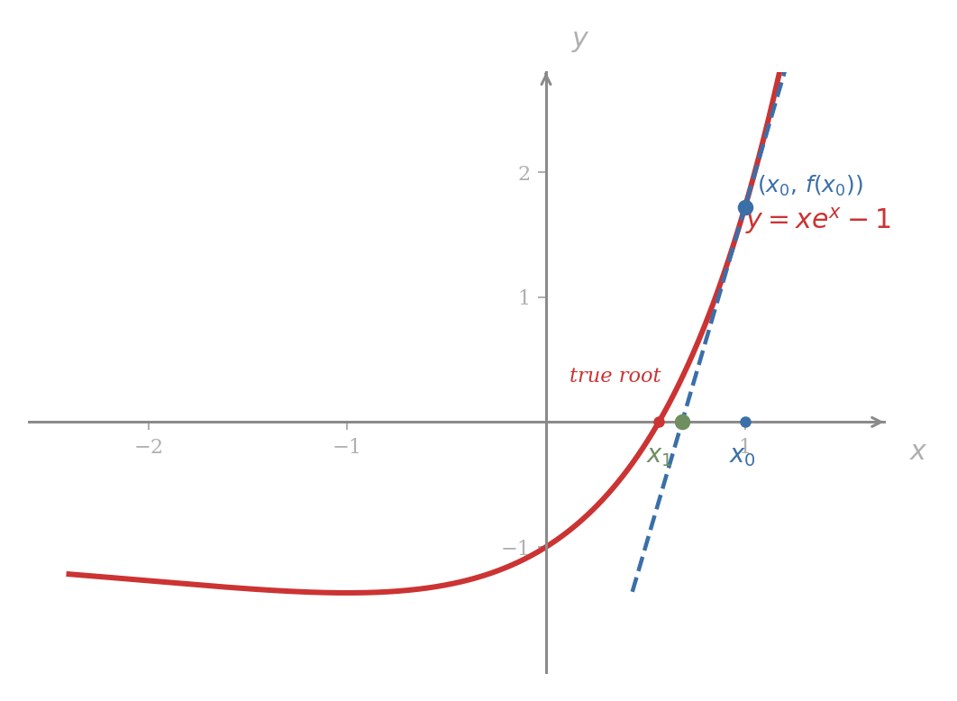
The Tangent-Line Trick

We pick any starting guess $x_{0}$ and look at the tangent line to $y = f(x)$ at the point $(x_{0}, f(x_{0}))$ . By the point-slope formula from Lesson 1AM, our tangent has equation

y = f(x_{0}) + f'(x_{0}) \, (x - x_{0}). \tag{3}

Setting $y = 0$ in $(3)$ gives us the $x$ -intercept of the tangent:

0 = f(x_{0}) + f'(x_{0}) \, (x - x_{0}), \qquad x = x_{0} - \frac{f(x_{0})}{f'(x_{0})}. \tag{4}

The right-hand side is defined whenever $f'(x_{0}) \neq 0$ . We call it $x_{1}$ .

The tangent line is the best linear approximation to $y = f(x)$ near $x_{0}$ that the derivative supplies us. If the curve is close to its tangent over the interval between $x_{0}$ and the true root, then $x_{1}$ is closer to the root than $x_{0}$ was. Repeating the construction with $x_{1}$ in place of $x_{0}$ produces $x_{2}$ , then $x_{3}$ , and so on.

Definition 42 (Newton's iteration)

Let $f$ be a differentiable function and $x_{0}$ a starting guess with $f'(x_{0}) \neq 0$ . The Newton iteration for $f$ from $x_{0}$ is the sequence $x_{0}, x_{1}, x_{2}, \dots$ defined by

x_{n+1} = x_{n} - \frac{f(x_{n})}{f'(x_{n})}, \tag{5}

provided $f'(x_{n}) \neq 0$ at every step.

Theorem 32 (Geometric reading of

(5)

)

$x_{n+1}$ is the $x$ -intercept of the tangent line to $y = f(x)$ at the point $(x_{n}, f(x_{n}))$ .

Proof

The tangent line to $y = f(x)$ at $x = x_{n}$ has equation

y = f(x_{n}) + f'(x_{n}) \, (x - x_{n})

by point-slope. Setting $y = 0$ and dividing by $f'(x_{n}) \neq 0$ gives $x = x_{n} - f(x_{n})/f'(x_{n})$ , which is $(5)$ .

■

The curve y = xe^x - 1 drawn solid in red. A starting point (x_0, f(x_0)) at x_0 = 1 sits above the x-axis at height e - 1 ≈ 1.72. The tangent line at that point, drawn dashed in blue, slopes upward to the right and meets the x-axis at x_1 ≈ 0.684, between the starting point and the true root marked at x ≈ 0.567.

If the linear approximation is good, $x_{1}$ has overshot the root by less than $x_{0}$ did, and each iterate sits closer to the root than the previous one.

A Worked Example: $x e^{x} = 1$

We rewrite equation $(1)$ as $f(x) = x \, e^{x} - 1 = 0$ . By the product rule applied to $x$ and $e^{x}$ , with the derivative $\dfrac{d}{dx}(e^{x}) = e^{x}$ from Lesson 5AM,

f'(x) = 1 \cdot e^{x} + x \cdot e^{x} = (x + 1) \, e^{x}. \tag{6}

Example 162 (Newton's method applied to

x e^{x} = 1

)

Apply Newton’s iteration from $x_{0} = 1$ and report the first few iterates to seven decimal places.

By $(5)$ with our explicit $f$ and $f'$ above,

x_{n+1} = x_{n} - \frac{x_{n} \, e^{x_{n}} - 1}{(x_{n} + 1) \, e^{x_{n}}}.

At $x_{0} = 1$ : $f(1) = e - 1$ , $f'(1) = 2 e$ , so

x_{1} = 1 - \frac{e - 1}{2 e} = 1 - \frac{1}{2} + \frac{1}{2 e} = \frac{1}{2} + \frac{1}{2 e} \approx 0.6839397.

Continuing the iteration with a calculator at each step:

$n$	$x_{n}$
$0$	$1.0000000$
$1$	$0.6839397$
$2$	$0.5774545$
$3$	$0.5672297$
$4$	$0.5671433$
$5$	$0.5671433$

Our iterates have stabilised at $x_{5} = x_{4}$ to seven decimal places. The truncated value $x \approx 0.5671433$ satisfies $x \, e^{x} \approx 1.0000000$ , with $f(0.5671433) \approx 2.65 \times 10^{-8}$ .

After only four iterations our digits stop changing. The number of correct decimals roughly doubles at each step: our gap between $x_{0}$ and the root has size $\sim 0.43$ , between $x_{1}$ and the root $\sim 0.12$ , between $x_{2}$ and $x_{3}$ the digits agree only at the first decimal, and by $x_{4}$ the agreement is at the seventh.

This doubling of correct decimals is the typical behaviour of Newton’s method when the starting guess is close enough to the root. A formal proof needs more of the linear-approximation theory than this lesson develops; the observation that each iteration roughly squares the previous error is enough to explain why we prefer Newton’s method to bisection in practice.

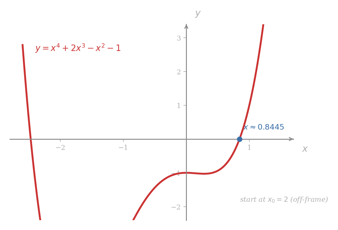
A Quartic Example

The polynomial $(2)$ has $f(x) = x^{4} + 2 x^{3} - x^{2} - 1$ , and by the Power and sum rules from Lesson 2PM

f'(x) = 4 x^{3} + 6 x^{2} - 2 x.

Example 163 (Newton's method on a quartic equation)

Apply Newton’s iteration to $f(x) = x^{4} + 2 x^{3} - x^{2} - 1 = 0$ from the starting guess $x_{0} = 2$ , in search of the unique positive root near $x \approx 0.8445$ .

A direct evaluation gives us $f(2) = 16 + 16 - 4 - 1 = 27$ and $f'(2) = 32 + 24 - 4 = 52$ , so

x_{1} = 2 - \frac{27}{52} \approx 1.4807692.

Continuing each step with a calculator:

$n$	$x_{n}$
$0$	$2.000000$
$1$	$1.480769$
$2$	$1.130977$
$3$	$0.930045$
$4$	$0.854880$
$5$	$0.844675$
$6$	$0.844499$

Our iterates converge on $x \approx 0.8445$ after six rounds. The first few rounds spend their effort closing the gap between $x_{0} = 2$ and the basin of fast convergence near the root; once we are close, the digits double per round, exactly as in the previous example.

Our starting guess $x_{0} = 2$ is a poor choice numerically, since $f(2) = 27$ is far from zero. A starting guess closer to the root, say $x_{0} = 1$ , would converge in fewer rounds: $f(1) = 1$ , $f'(1) = 8$ , $x_{1} = 1 - 1/8 = 0.875$ , and a few more rounds deliver the same accuracy.

The graph of y = x^4 + 2x^3 - x^2 - 1, drawn in red, crossing the x-axis at one positive root marked at x ≈ 0.8445 and at one negative root near x ≈ -2.47. The curve dips to a minimum below zero in the middle and climbs steeply upward on both sides.

Our two examples share the same arithmetic: every iteration is one evaluation of $f$ , one evaluation of $f'$ , and one division. Both use the toolkit we assembled in Lessons 4 and 5; nothing new about the operations themselves.

A Cube Root in Closed Form

The classical demonstration of Newton’s method is the computation of $\sqrt[3]{2}$ to many decimals, using only $+$ , $-$ , $\times$ , $\div$ .

Example 164 (The cube root of

2

)

Solve $x^{3} = 2$ by Newton’s method from $x_{0} = 1.5$ , and report the iterates to seven decimal places.

We set $f(x) = x^{3} - 2$ and $f'(x) = 3 x^{2}$ from the power rule of Lesson 2PM. Our iteration $(5)$ becomes

x_{n+1} = x_{n} - \frac{x_{n}^{3} - 2}{3 x_{n}^{2}} = \frac{2 x_{n}}{3} + \frac{2}{3 x_{n}^{2}},

where the simplification splits $x_{n} - x_{n}/3 = 2 x_{n}/3$ from the first term and isolates the constant $2/(3 x_{n}^{2})$ from the second.

The iterates from $x_{0} = 1.5$ :

x_{1} = 1.0 + \frac{2}{6.75} \approx 1.2962963, \quad x_{2} \approx 1.2609322, \quad x_{3} \approx 1.2599219, \quad x_{4} \approx 1.2599210.

By $x_{4}$ our iterates have stabilised at $\sqrt[3]{2} \approx 1.2599210$ , with $x_{4}^{3} - 2 \approx 4 \times 10^{-15}$ on a calculator that carries fifteen digits.

Our closed-form simplification $x_{n+1} = (2 x_{n})/3 + 2/(3 x_{n}^{2})$ admits the reading “two-thirds of the previous estimate plus one-third of the exact fix”: each iterate is a weighted average that gives more weight to the previous estimate but pulls partly toward the value that would solve the equation if the curve were genuinely linear at $x_{n}$ .

Problem 180

Use Newton’s method from $x_{0} = 2$ to compute $\sqrt[3]{5}$ to six decimal places. Show the simplified iteration formula in the form

x_{n+1} = \frac{2 x_{n}}{3} + \frac{5}{3 x_{n}^{2}},

and tabulate $x_{0}, x_{1}, x_{2}, x_{3}, x_{4}$ .

Problem 181

For the equation $f(x) = e^{x} - 3 x = 0$ , Newton’s method from $x_{0} = 1$ converges to one root and from $x_{0} = 2$ converges to another. Compute the first three iterates from each starting point to four decimal places, and identify the two roots numerically. Use the formula for the derivative of $e^{x}$ from Lesson 5AM.

When the Tangent Is Horizontal

Our iteration $(5)$ involves a division by $f'(x_{n})$ and breaks down whenever the tangent at $x_{n}$ is horizontal.

Example 165 (A starting point where

f' = 0

)

For $f(x) = x \, e^{x} - 1$ , the derivative $f'(x) = (x + 1) e^{x}$ from $(6)$ vanishes at $x = -1$ , since $e^{x}$ never vanishes and the factor $x + 1$ does. Starting Newton’s iteration from $x_{0} = -1$ produces

x_{1} = x_{0} - \frac{f(x_{0})}{f'(x_{0})} = -1 - \frac{-1/e - 1}{0},

which is undefined. Geometrically, the tangent at $(-1, -1/e - 1)$ is horizontal and never crosses the $x$ -axis.

Our remedy is a different starting guess. Any $x_{0}$ with $f'(x_{0}) \neq 0$ avoids the break-down. For this $f$ , the only $x$ at which $f'(x) = 0$ is $x = -1$ ; every other starting choice keeps our iteration well-defined.

A horizontal tangent is also a danger nearby, even when the starting iterate avoids the exact zero of $f'$ . The denominator in $(5)$ shrinks to nearly zero as $x_{n}$ approaches a critical number, blowing up the size of the correction $f(x_{n})/f'(x_{n})$ and throwing the next iterate far from where it would otherwise land.

A Starting Point That Wanders Off

Our other failure mode is more subtle: the iteration is well-defined at every step but moves away from the root. The shape of the curve far from the root determines whether this happens.

Example 166 (

x_{0} = -2

for

x e^{x} - 1

)

The same equation $x \, e^{x} = 1$ has its unique real root near $x \approx 0.5671$ . Starting Newton’s iteration from $x_{0} = -2$ :

f(-2) = -2 e^{-2} - 1 \approx -1.2707, \qquad f'(-2) = (-1) e^{-2} \approx -0.1353,

x_{1} = -2 - \frac{-1.2707}{-0.1353} \approx -2 - 9.39 = -11.39.

The next iterate is far further from the root than the start. Continuing,

x_{2} \approx -8516.92, \qquad x_{3} \approx \text{(further still, with magnitude growing)}.

The iterates diverge toward $-\infty$ .

The cause is visible in our curve $y = x e^{x} - 1$ : as $x \to -\infty$ , the term $x e^{x}$ shrinks to zero (the exponential decay overwhelms the linear factor), so $f(x) \to -1$ . The curve has the line $y = -1$ as a horizontal asymptote on the left. Newton’s iteration, looking at the gentle slope of the asymptotic region and assuming the curve is approximately linear, projects the tangent to a faraway intercept; our next iterate lands in even gentler asymptotic territory; and the process accelerates outward instead of homing in.

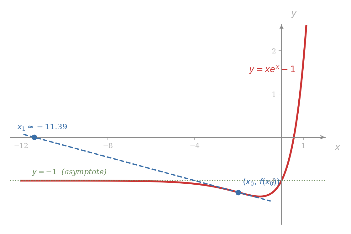
A wide-view graph of y = xe^x - 1 from x = -12 to x = 1.5. The curve sits very close to the dotted horizontal asymptote y = -1 across the entire negative region, then rises steeply in the rightmost portion to cross the x-axis. The tangent line at (-2, ≈ -1.27), drawn dashed, has very gentle negative slope and crosses the x-axis far to the left at x_1 ≈ -11.39.

The shallow slope of the tangent in the asymptotic region is the cause: dividing $f(x_{n}) \approx -1$ by a small $f'(x_{n}) \approx 0$ produces a large correction. Newton’s method needs more than $f'(x_{n}) \neq 0$ ; it needs a starting region where the curve is not too close to a horizontal asymptote.

Remark

The two failure cases just shown sit at opposite extremes:

Local horizontal tangent at the iterate ( $f'(x_{n}) = 0$ ): division by zero, the next iterate is undefined.
Far-asymptotic region ( $f(x_{n})$ close to a horizontal asymptote): division by a tiny number, the next iterate is huge and farther from the root.

Both are symptoms of the same tension: a shallow tangent line cannot be trusted to predict where the true curve crosses zero.

A Function with No Real Root

Newton’s method assumes that $f(x) = 0$ has a solution. When it does not, our iteration must do something with each $x_{n}$ , and the resulting sequence cannot converge to anything sensible.

Example 167 (

f(x) = x^{2} + 1

has no real root)

The function $f(x) = x^{2} + 1$ satisfies $f(x) \geq 1 > 0$ for every real $x$ , so there is no $x$ with $f(x) = 0$ . The Newton iteration formula

x_{n+1} = x_{n} - \frac{x_{n}^{2} + 1}{2 x_{n}}

is, however, defined whenever $x_{n} \neq 0$ . Starting from $x_{0} = 2$ gives the sequence

x_{1} = 2 - \frac{5}{4} = 0.75, \quad x_{2} \approx -0.2917, \quad x_{3} \approx 1.5685, \quad x_{4} \approx 0.4655,

x_{5} \approx -0.8415, \quad x_{6} \approx 0.1734, \quad x_{7} \approx -2.7970, \quad \dots

Our iterates oscillate without settling. Some sit close to the origin, others land well outside the interval $[-1, 1]$ , and the magnitudes occasionally swing into the threes. No sub-pattern repeats.

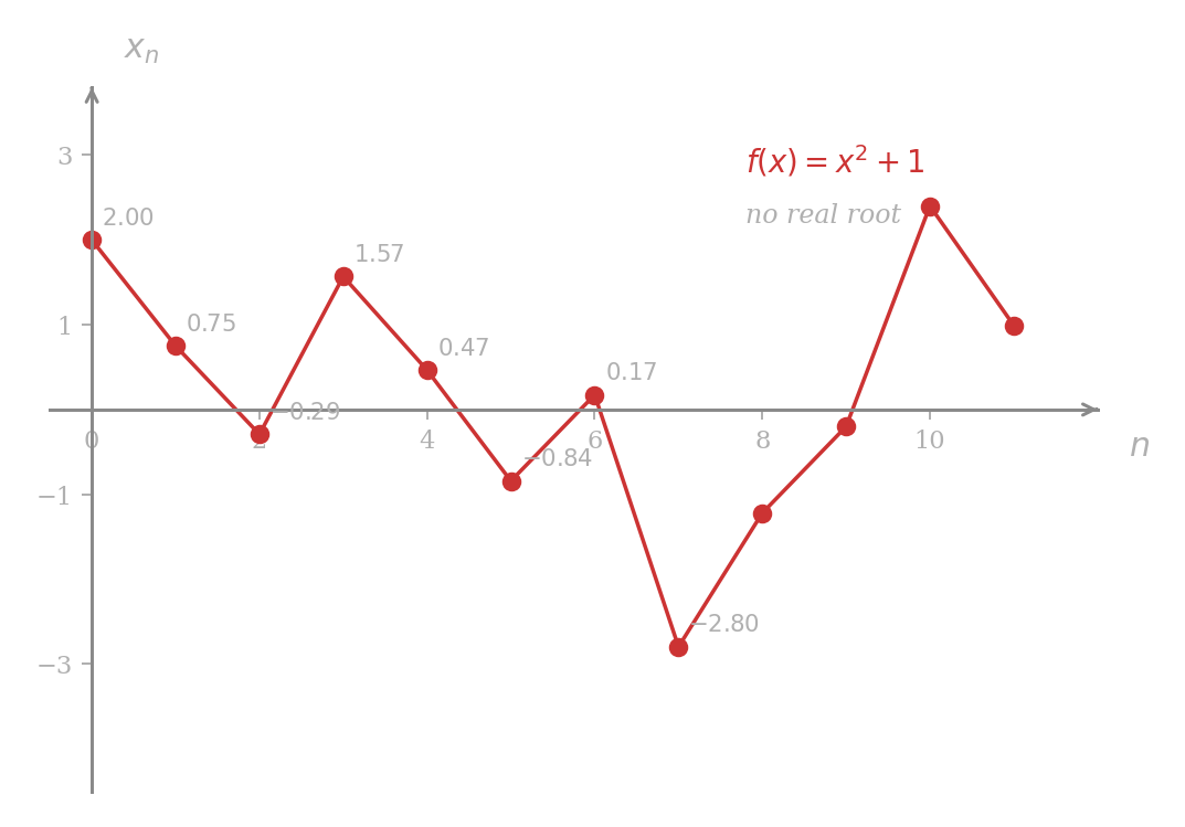
A line plot of x_n versus n for the Newton iteration on f(x) = x^2 + 1 starting from x_0 = 2. The points oscillate between positive and negative values without converging: 2.00, 0.75, -0.29, 1.57, 0.47, -0.84, 0.17, -2.80, and so on. A label notes 'no real root' to explain the absence of convergence.

A starting guess as close to the origin as $x_{0} = 1$ already runs into trouble of a different kind: the next iterate is

x_{1} = 1 - \frac{2}{2} = 0,

and $f'(0) = 0$ then forbids any further step. Different starting guesses produce different chaotic behaviours. The qualitative lesson: Newton’s method itself does not certify that a real solution exists; a graph or a separate sign check is still needed.

Problem 182

For the equation $\ln x = 1/x$ on $x > 0$ , define $f(x) = \ln x - 1/x$ . Compute $f'(x)$ using the derivative of $\ln$ from Lesson 5PM. Starting from $x_{0} = 2$ , perform Newton’s method to four decimal places and report the iterates $x_{0}, x_{1}, x_{2}, x_{3}$ . Confirm the iterates are settling by comparing successive values.

Problem 183

Apply Newton’s method to $f(x) = x^{3} - 3 x + 1$ on the real line. The cubic has three real roots, near $x \approx -1.879$ , $x \approx 0.347$ , and $x \approx 1.532$ .

Compute $f'(x)$ and identify the two values at which $f'(x) = 0$ . These are the values to avoid as starting guesses.
Starting from $x_{0} = -2$ , $x_{0} = 0$ , and $x_{0} = 2$ , perform three Newton iterations from each. Confirm that each starting guess converges to the nearest of the three roots.
Find a starting guess between $0$ and $1$ that converges to the negative root $x \approx -1.879$ rather than the nearby root at $x \approx 0.347$ , and explain in one sentence why such a starting guess exists. (Hint: pick a point at which the tangent is shallow but pointing leftward.)

Problem 184

A British project manager solves for the time $t > 0$ at which a mixed savings account, with balance

B(t) = 1000 \, e^{0.05 \, t} + 500 \, t,

first reaches £ $5\,000$ . The equation $B(t) - 5000 = 0$ has no closed-form solution.

Set $f(t) = 1000 \, e^{0.05 \, t} + 500 \, t - 5000$ . Compute $f'(t)$ using the formula for $e^{k x}$ .
Starting from $t_{0} = 5$ , perform Newton’s iteration to four decimal places. Tabulate $t_{0}, t_{1}, t_{2}, t_{3}, t_{4}$ .
Verify the answer by computing $B$ at the converged $t$ and confirming it is within £ $0.01$ of £ $5\,000$ .

Problem 185

(Harder.) For $f(x) = x \, e^{x} - 1$ from $(1)$ , the iteration $(5)$ takes the form

x_{n+1} = x_{n} - \frac{x_{n} \, e^{x_{n}} - 1}{(x_{n} + 1) \, e^{x_{n}}}.

Show that the right side simplifies to

x_{n+1} = \frac{x_{n}^{2}}{x_{n} + 1} + \frac{e^{-x_{n}}}{x_{n} + 1},

and identify each summand. The first term comes from the difference $x_{n} - x_{n}/(x_{n} + 1)$ ; the second comes from the constant $1/((x_{n}+1) e^{x_{n}})$ . Use the simplified formula to recompute $x_{1}$ from $x_{0} = 1$ and confirm $x_{1} = 1/2 + 1/(2 e)$ .

Problem 186

(Harder.) A function $f(x)$ is called monotonic on an interval if it is either strictly increasing or strictly decreasing on the interval. Suppose $f$ is differentiable, $f' > 0$ everywhere on an interval $[a, b]$ , and $f(a) < 0 < f(b)$ , so $f$ has a unique root $r$ in $(a, b)$ . Use the second derivative rule to argue that:

If $f''(x) \geq 0$ on $[a, b]$ (so $f$ is concave up there), then for every starting guess $x_{0}$ in $[a, b]$ with $x_{0} > r$ , the Newton iterates form a strictly decreasing sequence bounded below by $r$ .
If $f''(x) \leq 0$ on $[a, b]$ (so $f$ is concave down there), then for every starting guess $x_{0}$ in $[a, b]$ with $x_{0} < r$ , the Newton iterates form a strictly increasing sequence bounded above by $r$ .

(In each case the iterates approach the root from one side without overshoot. The general overshoot pattern of Newton’s method is therefore forbidden when the curve has the favourable concavity sign across the interval.)

Closing

Newton’s method is our last application of differentiation in this course. It uses every part of the toolkit we’ve built (the tangent-line construction from Lesson 2, the rules of differentiation from Lessons 4 and 5, the geometry of asymptotes from Lesson 3PM, and the rate-equation reading of $e^{r t}$ from Lesson 6AM) to turn an equation that resists algebra into a numerical procedure that converges in a handful of arithmetic steps.

Our next major question, taken up in MA0B, asks for the cumulative total of a function over an interval rather than the slope at a point. The two questions are connected, and the answer to the second turns out to involve the answer to the first in a way that justifies our entire derivative apparatus once more, but the development belongs to the integration course.

Note (Toolkit additions from this lesson)

Tool	Form
Newton’s iteration	$x_{n+1} = x_{n} - f(x_{n})/f'(x_{n})$
Geometric reading	$x_{n+1}$ is the $x$ -intercept of the tangent at $x_{n}$
Failure modes	$f'(x_{n}) = 0$ , asymptotic region, no real root