20/03/2026

#Math#Differentiation

Lesson assets

No linked assets.

Logarithmic Derivatives, Elasticity, and Bounded Growth

Lesson 5AM produced $y = C \, e^{k t}$ as the solution family of the rate equation $y' = k \, y$ , and Lesson 5PM introduced the derivative $\dfrac{d}{d x} \ln x = 1/x$ together with logarithmic differentiation. The chain rule applied to $\ln f$ recasts the same machinery in two further directions. The logarithmic derivative $f' / f$ measures a relative rate of change, which is the natural language for comparing percentage growth in economics and which gives the demand-side notion of elasticity. The substitution $u = M - y$ turns the rate equation into $u' = -k u$ , so the equation $y' = k(M - y)$ inherits a closed-form solution at no cost; this is the shape underlying bounded learning curves, mass-media diffusion of news, and the approach to steady state under intravenous infusion. This recitation applies both extensions, ending with the logistic family $y = M / (1 + B \, e^{-c t})$ .

The Logarithmic Derivative

For any positive differentiable $f$ , the chain rule for $\ln$ gives

\frac{d}{d t} \ln f(t) \;=\; \frac{f'(t)}{f(t)}.

The right side compares the rate of change $f'(t)$ to the current value $f(t)$ , so it has units of fraction per unit of $t$ . Multiplied by $100$ , the same quantity reads as a percentage.

Definition 1 (Relative and percentage rate of change)

The relative rate of change of a positive differentiable function $f$ at time $t$ is the logarithmic derivative

\frac{f'(t)}{f(t)} \;=\; \frac{d}{d t} \ln f(t).

Multiplied by $100$ , the same quantity is the percentage rate of change of $f$ at time $t$ .

An absolute change in money is meaningful only against an absolute base value. If beef costs $\pounds 5.25$ per kilogram and is rising at $\pounds 0.75$ per year while a car costs $\pounds 12\,000$ and is rising at $\pounds 1500$ per year, the slopes $0.75$ and $1500$ are not directly comparable. The percentages

\frac{0.75}{5.25} \approx 14.3\% \text{ per year}, \qquad \frac{1500}{12\,000} = 12.5\% \text{ per year}

are, and show that the beef price is rising slightly faster in relative terms than the car price.

Example 1 (A national-income model)

A simple model for a country’s gross domestic product, measured in trillions of pounds and timed in years from January 1, 1990, takes the form

N(t) \;=\; 4 + 0.05 \, t + 0.08 \, e^{-t}.

Find the percentage rate of change of $N$ on January 1, 1990, and on January 1, 1991.

By the sum rule and the formula for $e^{k t}$ with $k = -1$ ,

N'(t) \;=\; 0.05 - 0.08 \, e^{-t}.

The percentage rate of change is $N'(t)/N(t)$ . At $t = 0$ ,

\frac{N'(0)}{N(0)} \;=\; \frac{0.05 - 0.08}{4 + 0.08} \;=\; \frac{-0.03}{4.08} \;\approx\; -0.00735,

or about $-0.74\%$ per year; the economy is contracting. At $t = 1$ ,

\frac{N'(1)}{N(1)} \;=\; \frac{0.05 - 0.08 \, e^{-1}}{4.05 + 0.08 \, e^{-1}} \;\approx\; \frac{0.0206}{4.0794} \;\approx\; 0.00505,

or about $0.5\%$ per year; the economy is growing. The transient term $0.08 \, e^{-t}$ controls the early dynamics; once it has decayed, $N(t) \approx 4 + 0.05 \, t$ and the relative growth rate is approximately $0.05 / (4 + 0.05 \, t)$ , positive but slowly decreasing as $t$ grows.

Example 2 (Relative growth of an investment)

The value of a certain investment is modelled by

V(t) \;=\; 50\,000 \, e^{0.4 \sqrt{t}},

with $t$ in years. Use the logarithmic derivative to express the percentage rate of growth in closed form, and evaluate it at $t = 4$ and $t = 9$ years.

We take $\ln$ of both sides first; by LI and LIV from Lesson 5PM,

\ln V(t) \;=\; \ln 50\,000 + 0.4 \, t^{1/2}.

Differentiating, with the power rule,

\frac{V'(t)}{V(t)} \;=\; \frac{d}{d t} \!\left( \ln 50\,000 + 0.4 \, t^{1/2} \right) \;=\; \frac{0.2}{\sqrt{t}}.

At $t = 4$ the relative rate is $0.2/2 = 0.1$ , that is, $10\%$ per year. At $t = 9$ it is $0.2/3 \approx 6.7\%$ per year. The investment is still growing at every $t > 0$ , but its fractional growth rate falls toward zero as $t$ increases (a hallmark of $e^{a \sqrt{t}}$ that distinguishes it from pure exponential growth $e^{a t}$ , whose relative rate is the constant $a$ ).

Remark

Worked this way, the logarithmic derivative saves us the work of differentiating $V$ directly and then dividing: $V'$ would contain a stray factor of $V$ that immediately cancels. Our trick (take $\ln$ first, then differentiate) is exactly the logarithmic differentiation of Lesson 5PM, here serving as a measurement rather than as a simplification.

Note (Constant relative rate forces exponential growth)

If $f' / f = k$ for some constant $k$ , then $f' = k \, f$ , which is the rate equation of Lesson 5AM. Its solutions are $f(t) = C \, e^{k t}$ . A constant relative rate of change is therefore equivalent to exponential growth (or decay, when $k < 0$ ): there are no other functions with that property.

Problem 1

A country’s population is described by $P(t) = 200 \, e^{0.02 \, t} + 50 \, t$ , with $P$ in millions and $t$ in years from $1990$ .

Compute $P'(t)$ .
Find the percentage rate of growth at $t = 0$ and at $t = 25$ , in closed form, by evaluating $P'(t)/P(t)$ at each time.
As $t$ grows large, which of the two terms dominates $P(t)$ ? Use that to predict the long-run percentage rate of growth, and check the prediction against $P'(100)/P(100)$ .

Problem 2

The price-level index of a small economy is modelled by

I(t) \;=\; 100 \, e^{0.03 t} \, (1 + 0.1 \, t),

with $t$ in years.

Take $\ln I$ , then differentiate, to express $I'/I$ as a single closed-form expression without ever computing $I'$ directly.
Evaluate the percentage rate of change at $t = 0$ , $t = 5$ , and $t = 20$ .
Show that $I'/I \to 0.03 = 3\%$ as $t \to \infty$ , and explain in one sentence why the linear factor’s contribution vanishes.

Problem 3

A function $f$ satisfies $f(0) = 8$ and $f'(t)/f(t) = -0.25$ for every $t \geq 0$ .

Identify the ODE that $f$ satisfies and write its closed-form solution using the solutions theorem.
Find the time at which $f(t) = 1$ , in closed form involving $\ln 8$ .
Express the same time using $\ln 2$ instead.

Elasticity of Demand

A demand function expresses the quantity $q$ that a market will buy at price $p$ . We write $q = f(p)$ with $f$ positive and decreasing on the relevant range. Its derivative $f'(p)$ is negative, but for us the meaningful comparison is the relative rate of change $f'(p) / f(p)$ , which reads as quantity’s percentage response per unit of price.

The relative rate of change of price itself, with respect to $p$ , is

\frac{1}{p} \cdot \frac{d}{d p}(p) \;=\; \frac{1}{p}.

Our ratio of the two relative rates is

\frac{f'(p)/f(p)}{1/p} \;=\; \frac{p \, f'(p)}{f(p)}.

This quantity is negative for every decreasing demand function, so economists multiply by $-1$ to keep their bookkeeping positive.

Definition 2 (Elasticity of demand)

For a demand function $q = f(p)$ with $p > 0$ , $f(p) > 0$ , and $f'(p) < 0$ , the elasticity of demand at price $p$ is

E(p) \;=\; -\,\frac{p \, f'(p)}{f(p)}.

Demand is elastic at $p_{0}$ when $E(p_{0}) > 1$ and inelastic when $E(p_{0}) < 1$ .

Example 3 (Elasticity for a linear demand)

The demand for a certain metal is $q = 100 - 2 p$ (in millions of kilograms) at price $p$ pounds per kilogram, with $0 < p < 50$ .

Compute $E(p)$ in closed form.
Evaluate $E(30)$ and $E(20)$ , and interpret each.
Find the price at which $E(p) = 1$ .

With $f(p) = 100 - 2 p$ , $f'(p) = -2$ , so

E(p) \;=\; -\,\frac{p \cdot (-2)}{100 - 2 p} \;=\; \frac{2 p}{100 - 2 p}.

At $p = 30$ , $E(30) = 60/(100 - 60) = 60/40 = 1.5$ . A $1\%$ price increase from $\pounds 30$ per kilogram will reduce quantity demanded by about $1.5\%$ . Demand is elastic.

At $p = 20$ , $E(20) = 40/(100 - 40) = 40/60 = 2/3$ . A $1\%$ price increase from $\pounds 20$ will reduce quantity demanded by only about $0.67\%$ . Demand is inelastic.

The unit-elastic price solves $2 p / (100 - 2 p) = 1$ , that is, $2 p = 100 - 2 p$ , so $p = 25$ .

The economic significance of elasticity is its tie to revenue. With $R(p) = p \, f(p)$ , by the product rule,

R'(p) \;=\; f(p) + p \, f'(p) \;=\; f(p) \!\left[ 1 + \frac{p \, f'(p)}{f(p)} \right] \;=\; f(p) \,\bigl[ 1 - E(p) \bigr].

Since $f(p) > 0$ , the sign of $R'(p)$ matches the sign of $1 - E(p)$ :

where demand is elastic ( $E > 1$ ), $R'(p) < 0$ , so a price increase lowers revenue;
where demand is inelastic ( $E < 1$ ), $R'(p) > 0$ , so a price increase raises revenue.

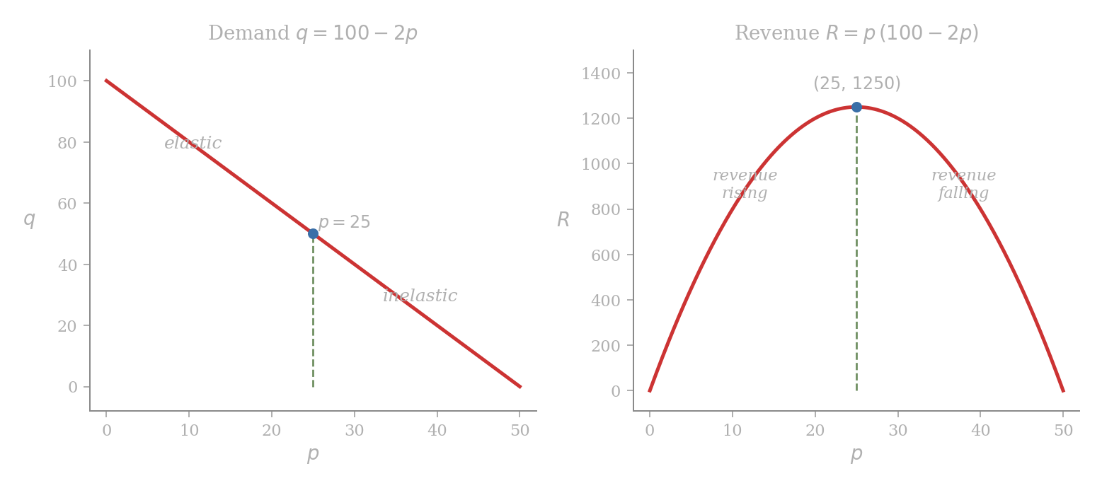
On the left, the linear demand curve q = 100 - 2p from p = 0 to p = 50, with a dashed vertical line at the unit-elastic price p = 25 and the regions labelled 'elastic' (p > 25) and 'inelastic' (p < 25). On the right, the revenue parabola R = p(100 - 2p) opening downward with its peak (25, 1250) marked, and arrows showing revenue rising for p < 25 and falling for p > 25.

The revenue parabola peaks at exactly $p = 25$ , the unit-elastic price. The second derivative test confirms the peak: $R(p) = 100 p - 2 p^{2}$ , $R'(p) = 100 - 4 p$ , $R''(p) = -4 < 0$ everywhere, so the unique critical point $p = 25$ is a global maximum on the relevant range.

Problem 4

For the demand function $q = 200 - 4 p$ on $0 \leq p \leq 50$ , compute elasticity for $0 < p < 50$ :

Find $E(p)$ in closed form.
Evaluate $E(20)$ and $E(40)$ , and state whether demand is elastic or inelastic at each.
Find the price at which $E(p) = 1$ , and verify it is the price at which the revenue $R(p) = p \, q$ is maximised.

Problem 5

The demand for a fashion item is $q = 600 \, e^{-0.05 \, p}$ at price $p$ pounds.

Use the logarithmic-derivative form to show that $E(p) = 0.05 \, p$ .
Find the price at which demand is unit-elastic.
Compute the elasticity at $p = 10$ and at $p = 30$ , and interpret each.

Problem 6

A demand function $q = f(p)$ has constant elasticity $E(p) = a$ for every $p > 0$ , where $a$ is a positive constant.

Rewrite the elasticity condition as the logarithmic-derivative equation $\dfrac{d}{d p} \ln f(p) = -a / p$ .
Verify directly, by computing $\dfrac{d}{d p} \ln(K p^{-a})$ using LI and LIV, that $f(p) = K \, p^{-a}$ satisfies this equation for every positive constant $K$ .
For $a = 1$ , show that the revenue $R(p) = p \, f(p)$ is constant on the entire domain.

Bounded Growth: the Family $y' = k(M - y)$

A natural variant of $y' = k y$ replaces the right side with $k (M - y)$ , where $M > 0$ and $k > 0$ are fixed constants. The variable $M$ acts as a ceiling: our rate of change is proportional to how far $y$ still lies below $M$ , so growth is fastest when $y$ is small and tapers off as $y$ approaches $M$ .

We let $u = M - y$ . Then $u' = -y'$ , and so

y'(t) \;=\; k \, (M - y(t)) \qquad \text{becomes} \qquad u'(t) \;=\; -k \, u(t).

The right-hand equation is the rate equation of Lesson 5AM with growth constant $-k$ . By the solutions theorem, $u(t) = A \, e^{-k t}$ for some constant $A$ , and therefore

y(t) \;=\; M - A \, e^{-k t}.

If $y(0) = 0$ , then $A = M$ and the closed form simplifies to $y(t) = M(1 - e^{-k t})$ .

Theorem 1 (Solutions of

y' = k(M - y)

)

For fixed constants $k > 0$ and $M > 0$ , every solution of

y'(t) \;=\; k \, (M - y(t))

has the form $y(t) = M - A \, e^{-k t}$ for some constant $A$ . The solution with $y(0) = 0$ is

y(t) \;=\; M \, (1 - e^{-k t}).

When $0 \leq y(0) < M$ , the curve grows upward toward the ceiling $M$ . If the starting value is already above $M$ , the same formula describes decay down toward $M$ instead.

Proof

Our substitution $u = M - y$ above converts the ODE into $u' = -k u$ , whose solutions are $u(t) = A \, e^{-k t}$ by Lesson 5AM. Hence $y(t) = M - A \, e^{-k t}$ . The initial condition $y(0) = 0$ gives $M - A = 0$ , so $A = M$ and $y(t) = M(1 - e^{-k t})$ .

To verify the differential equation directly, differentiate $y(t) = M - A \, e^{-k t}$ by the formula for $e^{k x}$ : $y'(t) = k A \, e^{-k t}$ . On the other hand $k(M - y(t)) = k \, A \, e^{-k t}$ . The two expressions agree.

■

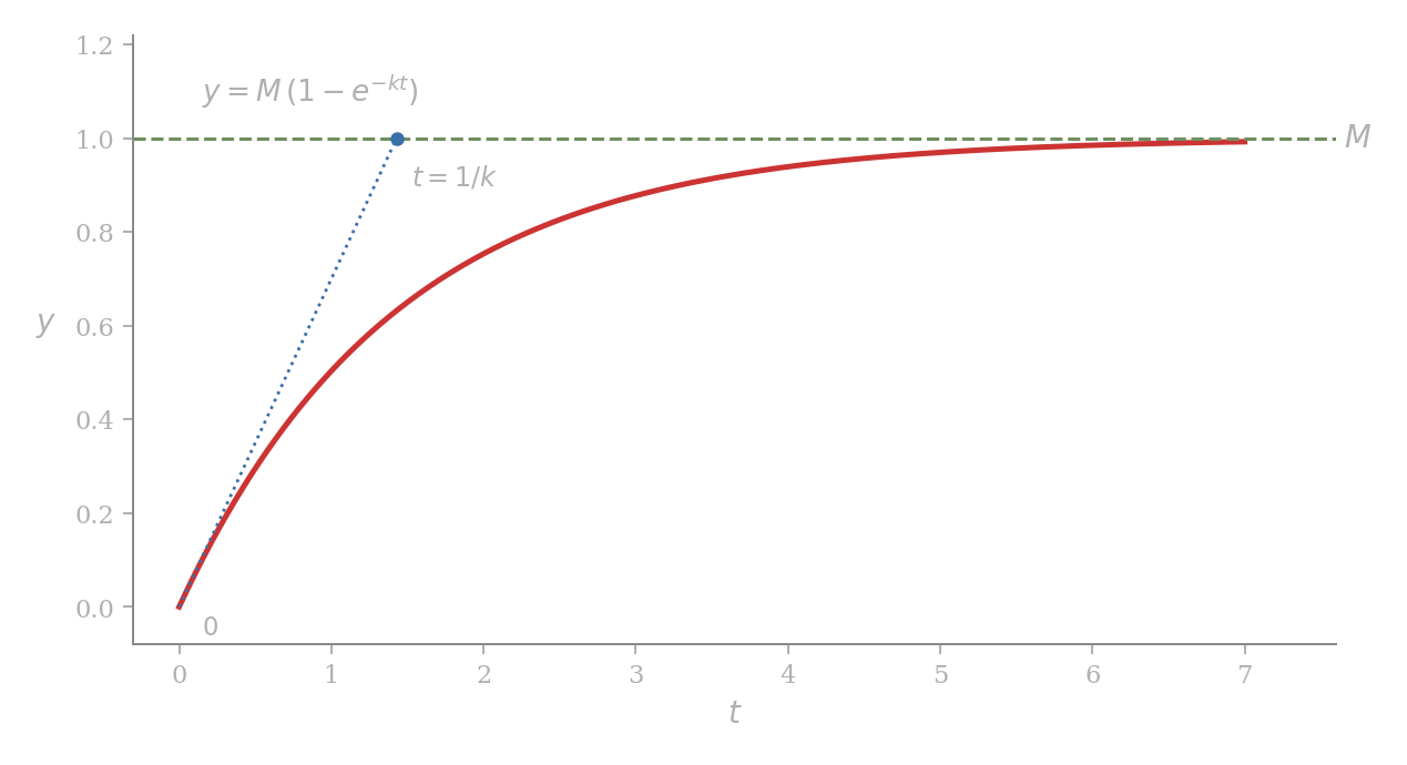
$The bounded-growth curve y = M(1 - e^{-kt}) starting at the origin, rising concave down, and approaching the dashed horizontal line y = M from below without ever reaching it. The initial tangent line is drawn dotted; it meets the line y = M at the point t = 1/k.$

Three numerical features of our curve $y = M(1 - e^{-k t})$ follow at once, mirroring the time-constant analysis of Lesson 5R:

The initial slope $y'(0) = k M$ is the largest slope of the curve, since $y'(t) = k M e^{-k t}$ decreases in $t$ .
The tangent at $t = 0$ meets the line $y = M$ at $t = 1/k$ ; the curve at that time has height $M(1 - e^{-1}) \approx 0.632 \, M$ .
$y(t) \to M$ as $t \to \infty$ ; the curve never reaches the ceiling but settles arbitrarily close to it.

Example 4 (Learning curve for nonsense syllables)

In a controlled experiment, a subject can memorise at most $M = 80$ nonsense syllables in a row given enough study time. After $t$ minutes of study the subject can correctly memorise $f(t)$ syllables, and $f$ satisfies

f'(t) \;=\; k \, (M - f(t)), \qquad f(0) = 0.

The subject can memorise $40$ syllables after $10$ minutes. Find $k$ and predict the number retained after $30$ minutes of study.

By the theorem, $f(t) = 80 \, (1 - e^{-k t})$ . The reading at $t = 10$ gives

80 \, (1 - e^{-10 k}) \;=\; 40, \qquad e^{-10 k} \;=\; \tfrac{1}{2}.

Taking $\ln$ and applying LII,

-10 k \;=\; -\ln 2, \qquad k \;=\; \frac{\ln 2}{10}.

With this $k$ ,

f(30) \;=\; 80 \, (1 - e^{-3 \ln 2}) \;=\; 80 \, (1 - 2^{-3}) \;=\; 80 \cdot \tfrac{7}{8} \;=\; 70.

The subject can memorise $70$ syllables after $30$ minutes, three half-lives of the deficit $M - f(t)$ removed from the initial gap of $80$ syllables.

Remark

If we reframe this as ” $10$ minutes of study halves the remaining gap,” our problem turns into a half-life problem in disguise: the deficit $M - f(t) = M \, e^{-k t}$ is itself a pure exponential decay with the same constant $k = (\ln 2)/10$ . Lessons 5PM and 5R apply unchanged to that deficit.

Example 5 (Diffusion of news by mass media)

In a city of $P$ residents, news of a public official’s resignation is broadcast continuously by radio and television. The number $f(t)$ of residents who have heard the news by time $t$ (in hours) satisfies

f'(t) \;=\; k \, (P - f(t)), \qquad f(0) = 0,

because the rate at which new people hear is proportional to the number who have not yet heard. Half of the residents have heard the news $4$ hours after release. When will $90\%$ have heard?

By the theorem, $f(t) = P \, (1 - e^{-k t})$ . The half-population condition at $t = 4$ gives $1 - e^{-4 k} = 1/2$ , so $e^{-4 k} = 1/2$ and $k = (\ln 2)/4$ .

The $90\%$ threshold solves

1 - e^{-k t} \;=\; 0.9, \qquad e^{-k t} \;=\; 0.1.

Taking $\ln$ ,

-k t \;=\; -\ln 10, \qquad t \;=\; \frac{\ln 10}{k} \;=\; \frac{4 \, \ln 10}{\ln 2} \;\approx\; \frac{4 \cdot 2.303}{0.693} \;\approx\; 13.3 \text{ hours}.

About $13$ hours after release, $90\%$ of the city has heard the news.

Problem 7

A patient receives a continuous intravenous infusion of glucose. The excess glucose level $A(t)$ above the equilibrium satisfies

A'(t) \;=\; r - \lambda \, A(t), \qquad A(0) = 0,

where $r$ is the (constant) rate of infusion in milligrams per minute and $\lambda > 0$ is the metabolic clearance constant.

Rewrite the ODE as $A'(t) = \lambda \, (M - A(t))$ , identifying $M$ in terms of $r$ and $\lambda$ .
Use the bounded-growth theorem to write $A(t)$ in closed form.
With $r = 60$ mg/min and $\lambda = 0.02$ per minute, find the limiting level $M$ , then find the time at which $A(t)$ first reaches $0.9 M$ , in closed form involving $\ln 10$ .

Problem 8

A skydiver’s downward velocity $v(t)$ satisfies $v'(t) = k (M - v(t))$ with $v(0) = 0$ , where $M$ is the terminal velocity and $k > 0$ . The skydiver’s velocity reaches half of terminal in $4$ seconds.

Find $k$ in closed form involving $\ln 2$ .
Find the time at which the velocity first reaches $0.99 \, M$ .
Show that the acceleration $v'(t)$ is itself a pure exponential decay $k M \, e^{-k t}$ , and identify its half-life.

Problem 9

For the bounded-growth family $y(t) = M(1 - e^{-k t})$ :

Compute $y'(t)$ and $y''(t)$ in closed form. Confirm $y'$ is everywhere positive and $y''$ everywhere negative on $t \geq 0$ .
Find the relative rate of change $y'/y$ in closed form, and show it is not constant in $t$ , unlike for pure exponential growth.
Show that on any interval $[a, a + (\ln 2)/k]$ , $y$ covers exactly half of the gap remaining at the start of the interval. (Bounded growth as “half-of-what’s-left”.)

Logistic Growth

Our bounded-growth family handles populations that fill toward a ceiling at a rate proportional to the remaining gap. We meet a different shape (the S-curve) when the growth rate is also throttled by the size of the population itself in the early stage: a small population produces few offspring even with abundant resources, and an almost-full population grows slowly because the ceiling is near. The two effects together give us the logistic family

y(t) \;=\; \frac{M}{1 + B \, e^{-c t}},

with positive constants $M$ , $B$ , $c$ . As $t \to \infty$ , $e^{-c t} \to 0$ and $y \to M$ ; at $t = 0$ , $y(0) = M / (1 + B)$ , which is small whenever $B$ is large.

Theorem 2 (The logistic ODE)

The logistic function $y(t) = M / (1 + B \, e^{-c t})$ satisfies

y'(t) \;=\; \frac{c}{M} \, y(t) \, \bigl( M - y(t) \bigr).

Proof

We write $u = 1 + B \, e^{-c t}$ , so $y = M / u$ and $u'(t) = -c B \, e^{-c t}$ . By the chain rule,

y'(t) \;=\; -\frac{M}{u^{2}} \cdot u'(t) \;=\; \frac{M \, c \, B \, e^{-c t}}{u^{2}}.

On the other hand, using $u - 1 = B \, e^{-c t}$ ,

M - y \;=\; M - \frac{M}{u} \;=\; \frac{M(u - 1)}{u} \;=\; \frac{M \, B \, e^{-c t}}{u},

\frac{c}{M} \, y \, (M - y) \;=\; \frac{c}{M} \cdot \frac{M}{u} \cdot \frac{M \, B \, e^{-c t}}{u} \;=\; \frac{M \, c \, B \, e^{-c t}}{u^{2}},

which matches $y'(t)$ .

■

$The logistic S-curve y = M/(1 + Be^{-ct}) starting near zero, rising sharply through the inflection point at the height y = M/2, and flattening toward the dashed asymptote y = M. The inflection point is marked with a dot, and the level y = M/2 is shown as a dotted horizontal line.$

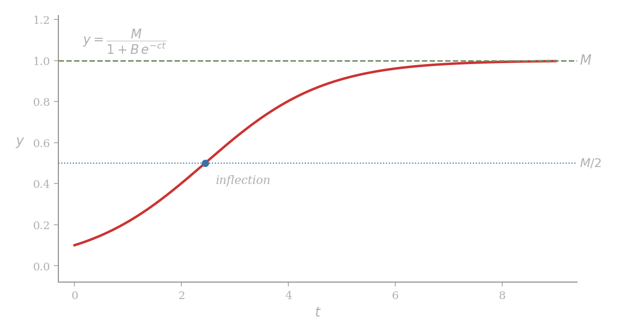
The right side of our logistic ODE is largest when the quadratic $y(M - y)$ is largest. That product, viewed as a function of $y$ , is maximised at $y = M/2$ . So the logistic curve grows fastest at exactly half-capacity, and its graph has an inflection point at $y = M/2$ . Solving $1 + B \, e^{-c t} = 2$ gives us the time of inflection $t = (\ln B) / c$ .

Example 6 (Fish stocked in a lake)

A lake is stocked with $100$ fish. Three months later there are $250$ fish. An ecological study predicts the lake can support a long-run population of $1000$ fish. Find a closed-form $P(t)$ for the population $t$ months after stocking, using the logistic model with ceiling $M = 1000$ .

By the logistic form,

P(t) \;=\; \frac{1000}{1 + B \, e^{-c t}}.

Our initial condition $P(0) = 100$ gives

100 \;=\; \frac{1000}{1 + B}, \qquad 1 + B \;=\; 10, \qquad B \;=\; 9.

The reading at $t = 3$ gives

250 \;=\; \frac{1000}{1 + 9 \, e^{-3 c}}, \qquad 1 + 9 \, e^{-3 c} \;=\; 4, \qquad e^{-3 c} \;=\; \tfrac{1}{3}.

Taking $\ln$ and applying LII gives $-3 c = -\ln 3$ , so $c = (\ln 3)/3 \approx 0.366$ . Therefore

P(t) \;=\; \frac{1000}{1 + 9 \, e^{-(\ln 3 / 3) \, t}}.

The inflection point (the moment of fastest growth) occurs at

t \;=\; \frac{\ln 9}{c} \;=\; \frac{2 \, \ln 3}{(\ln 3) / 3} \;=\; 6 \text{ months},

at which time $P = 500$ fish. After month $6$ , growth slows.

Example 7 (Spread of an epidemic)

In a city of $P = 500\,000$ residents, an epidemic of a long-lasting flu is monitored. At the start of the first week, $200$ cases are known, and $300$ new cases are reported during the first week. Using the logistic model

f(t) \;=\; \frac{P}{1 + B \, e^{-c t}},

estimate the number of infected residents at the end of the sixth week.

The condition $f(0) = 200$ gives

200 \;=\; \frac{500\,000}{1 + B}, \qquad 1 + B \;=\; 2500, \qquad B \;=\; 2499.

At $t = 1$ , $f(1) = 500$ :

500 \;=\; \frac{500\,000}{1 + 2499 \, e^{-c}}, \qquad 1 + 2499 \, e^{-c} \;=\; 1000, \qquad e^{-c} \;=\; \frac{999}{2499} = \frac{333}{833}.

So $c = \ln(833/333) \approx 0.9169$ . At $t = 6$ ,

f(6) \;=\; \frac{500\,000}{1 + 2499 \, e^{-6 c}} \;\approx\; 44\,600.

About $45\,000$ residents are infected after six weeks.

Remark

The logistic family is used by sociologists for the spread of a rumour and by economists for the diffusion of knowledge about a new product, with an “infected” individual representing one who has heard the rumour or knows the product. The spreading mechanism is interpersonal contact rather than mass media; the mass-media setting of the previous section uses the bounded-growth family $y' = k(M - y)$ instead. Bounded growth has no inflection point: its slope is largest at $t = 0$ and decreases monotonically.

Problem 10

For the logistic function $y(t) = M / (1 + B \, e^{-c t})$ with $M, B, c > 0$ :

Show $y(0) = M / (1 + B)$ and that $y(t) \to M$ as $t \to \infty$ .
Show the inflection point of $y$ occurs at $t = (\ln B) / c$ , at height $y = M/2$ .
Show the maximum growth rate is $y'_{\max} = c \, M / 4$ , attained at the inflection point.

Problem 11

A fruit-fly culture follows the logistic model with capacity $M = 1000$ . The culture starts with $50$ flies and reaches $200$ flies after $5$ days.

Determine $B$ from the initial condition.
Determine $c$ from the reading at $t = 5$ , in closed form.
Find the time at which the population first reaches $500$ (the inflection point), and check it equals $(\ln B)/c$ from part 1 of the previous problem.

Exercises

Exercise 1

A start-up’s revenue is modelled by $R(t) = 2 t \, e^{0.1 \, t}$ in millions of pounds, with $t$ in years from the founding.

Compute $R'(t)$ by the product rule.
Take $\ln R$ and differentiate to express $R'(t)/R(t)$ as a single closed-form expression.
Find every $t > 0$ at which the percentage rate of growth equals exactly $20\%$ per year, in closed form.

Exercise 2

The demand for a particular software licence is $q = 1000 - 5 p^{2}$ at price $p$ pounds, valid on $0 \leq p \leq 14$ .

Find $E(p)$ in closed form and show $E(p) = 2 p^{2} / (200 - p^{2})$ .
Find the price at which demand is unit-elastic, in closed form.
The price is currently $p_{0} = 8$ . Is demand elastic or inelastic at $p_{0}$ ? Will a small price increase from $p_{0}$ raise or lower revenue? Justify with the identity $R'(p) = f(p) (1 - E(p))$ .

Exercise 3

For the demand $q = 50 / p$ on $p > 0$ :

Compute $E(p)$ in closed form and verify that elasticity is constant in $p$ .
Conclude that revenue $R(p) = p \, q$ has the same value at every price $p > 0$ , and compute that value.
State, for a general demand of the form $f(p) = K \, p^{-a}$ with $K, a > 0$ , the elasticity $E(p)$ in closed form, and explain in one sentence why $a = 1$ is the dividing case between rising and falling revenue.

Exercise 4

A city’s monthly volume of landfill waste follows

W(t) \;=\; M - (M - W_{0}) \, e^{-k t}

where $W(0) = W_{0}$ , $M$ is the long-run steady-state value, and $k > 0$ .

Verify $W$ satisfies $W'(t) = k \, (M - W(t))$ for any choice of $W_{0}$ .
The city’s data are $W_{0} = 200$ tonnes, $M = 800$ tonnes, and $W(12) = 500$ tonnes (one year after monitoring began). Find $k$ in closed form involving $\ln 2$ .
Find the time at which $W$ first reaches $700$ tonnes.

Exercise 5

A glucose IV is set to a fixed rate $r$ , with metabolic clearance constant $\lambda$ . The excess glucose satisfies

A'(t) \;=\; r - \lambda \, A(t), \qquad A(0) = 0,

and we write $M = r/\lambda$ .

State $A(t)$ in closed form using the bounded-growth theorem.
The IV is shut off at time $T$ , at which point $A(T) = (3/4) M$ . After shutoff the body clears glucose with the same constant $\lambda$ , so the post-shutoff dynamics are $A'(t) = -\lambda \, A(t)$ . Find $\lambda T$ in closed form involving $\ln 4$ .
Express the time required, after shutoff, for the excess glucose to fall back to $0.1 \, M$ , in closed form involving $\ln$ .

Exercise 6

A bounded-growth process and a pure exponential decay are connected. Let $y(t) = M(1 - e^{-k t})$ be the bounded growth, and let $g(t) = M - y(t)$ be the residual gap.

Show $g$ satisfies $g'(t) = -k \, g(t)$ with $g(0) = M$ (pure exponential decay).
State the half-life of $g$ in closed form, and show it equals the time at which $y$ first reaches $M/2$ .
Show that on any interval $[a, a + T_{1/2}]$ with $T_{1/2} = (\ln 2)/k$ , the curve $y$ covers exactly half of the deficit remaining at the start of the interval, regardless of $a$ .

Exercise 7

In the early stage of logistic growth, when $y$ is small compared with $M$ , the logistic ODE

y'(t) \;=\; \frac{c}{M} \, y \, (M - y)

nearly coincides with a pure exponential growth equation.

Show that if $y(t) / M$ is negligible compared with $1$ , then $y'(t) \approx c \, y(t)$ .
Conclude that the logistic curve initially looks like a pure exponential with growth constant $c$ , and verify this by computing $y'(0)/y(0)$ in closed form for the logistic family $y(t) = M / (1 + B \, e^{-c t})$ .
Show that $y'(0)/y(0)$ approaches $c$ as $B \to \infty$ , that is, when the initial population is a very small fraction of the ceiling.

Exercise 8

A rumour spreads through a community of $P = 10\,000$ people according to the logistic model with parameters $B$ and $c$ . Initially $50$ people know the rumour; after $2$ days, $500$ know.

Determine $B$ from the initial condition.
Determine $c$ in closed form involving $\ln$ .
Estimate the day on which the rate of new infections is maximal, and the cumulative number of people who know the rumour on that day.

Exercise 9

A demand function $q = f(p)$ on $p > 0$ has $E(p) = 1 + p$ . Show that $f(p) = K \, e^{-p} / p$ satisfies this elasticity condition for every positive constant $K$ , by computing $-\, p \, f'(p) / f(p)$ directly for this $f$ and verifying that the result equals $1 + p$ .

Lesson assets

Logarithmic Derivatives, Elasticity, and Bounded Growth

The Logarithmic Derivative

Elasticity of Demand

Bounded Growth: the Family y′=k(M−y)y' = k(M - y)y′=k(M−y)

Logistic Growth

Exercises

Bounded Growth: the Family $y' = k(M - y)$