16/03/2026

#Math#Differentiation

Video

Lesson assets

video link

CS50P Lecture 0: Functions, Variables

exercise

Exercise 6 PDF

Continuous Compound Interest

In Recitation 4 we first met the $15\%$ investment as a single number multiplied year on year: the balance at the end of year $t$ was $1000 \cdot (1.15)^{t}$ , with the assumption that interest is paid once and added to the principal at year-end. Lesson 5AM lifted that model to a continuous-rate equation $B'(t) = k \, B(t)$ , and Lesson 5PM named our proportionality constant $k = \ln 1.15$ via the reduction theorem. We’ve suppressed two pieces of the picture so far: a real bank does not pay interest only at year-end, and the relationship between an advertised annual rate and our closed-form constant $k$ depends on how often the interest is added.

A bank that quotes an annual rate $r$ , written as a decimal, and compounds $m$ times per year applies the rate $r/m$ at each compounding step and credits the result to the balance. Increasing $m$ at a fixed $r$ increases the balance at the end of the year, but only by an amount that shrinks with $m$ . The limit of that process gives us the continuous compound formula, and our constant $k$ in $B(t) = P e^{k t}$ for that limit is exactly the advertised rate $r$ .

Compounding $m$ Times per Year

Let $P$ pounds be invested at an annual rate of $r$ (written as a decimal, so $6\%$ means $r = 0.06$ ), compounded $m$ times per year for $t$ years. Each compounding step multiplies the balance by $1 + r/m$ , and there are $m t$ such steps in $t$ years.

Theorem 29 (Discrete compound interest)

The compound amount $A$ after $t$ years at annual rate $r$ compounded $m$ times per year on an initial principal of $P$ pounds is

A = P \!\left(1 + \frac{r}{m}\right)^{\!m t}. \tag{1}

For £ $1000$ at $6\%$ over one year ( $P = 1000$ , $r = 0.06$ , $t = 1$ ), formula $(1)$ evaluated at four common choices of $m$ produces the table below.

Compounding	$m$	Balance after $1$ year (£)
Annually	$1$	$1060.00$
Quarterly	$4$	$1061.36$
Monthly	$12$	$1061.68$
Daily (360-day year)	$360$	$1061.83$

The annual figure £ $1060.00$ is the textbook simple-interest case. Quarterly compounding adds £ $1.36$ , monthly compounding adds another £ $0.32$ , and daily compounding adds a further £ $0.15$ . Each refinement of the schedule shrinks our gain. The next question is what happens at $m = \infty$ .

Balance after 1 year on £1000 at 6%, plotted against log_10(m). Eight points for m = 1, 2, 4, 12, 52, 360, 8760, 525600 lie along a smooth curve that rises sharply at first and flattens toward a horizontal asymptote at Pe^r ≈ 1061.84.

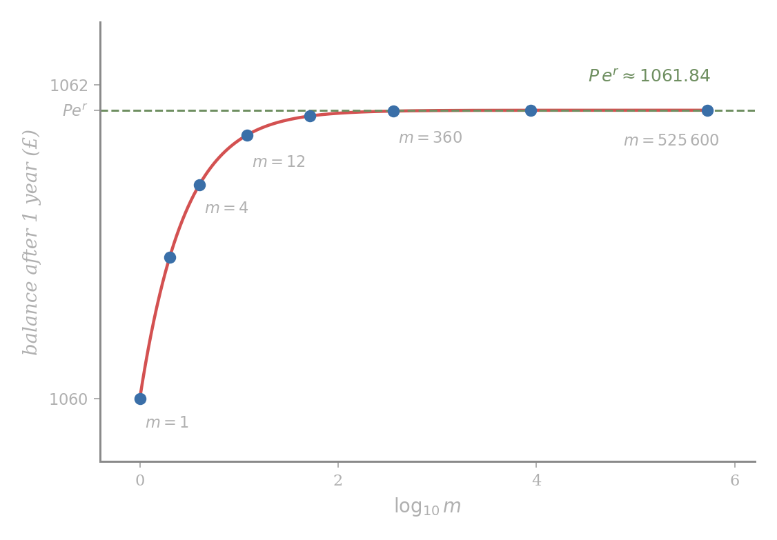
The points crowd toward an asymptote as $m$ grows. Going from annually to daily compounding gains £ $1.83$ ; going from daily to compounding once per second adds less than £ $0.01$ . The limit is in plain sight, but a formula for it requires the continuity of $\ln$ and the derivative computation from Lesson 5PM.

The Limit as $m \to \infty$

We rewrite $(1)$ to expose the structure of the exponent. With $h = r/m$ , our substitution gives $1/h = m/r$ and so $m t = (1/h) \cdot r t$ . Then

A = P \!\left(1 + \frac{r}{m}\right)^{\!m t} = P \!\left(1 + h\right)^{\!(1/h) \cdot r t}. \tag{2}

Sending $m \to \infty$ at fixed $r > 0$ sends $h = r/m \to 0$ through positive values, and our limit on the right of $(2)$ depends on the inner factor $(1 + h)^{1/h}$ alone.

Theorem 30 (A limit formula for

e

)

\lim_{h \to 0} (1 + h)^{1/h} = e. \tag{3}

Proof

For $h$ near $0$ but $h \neq 0$ , the base $1 + h$ is positive, and the real-power definition from Lesson 5PM applies:

(1 + h)^{1/h} = e^{(1/h) \ln(1 + h)}.

Since the exponential function is continuous,

\lim_{h \to 0} (1 + h)^{1/h} = \lim_{h \to 0} e^{(1/h) \ln(1 + h)} = e^{\,L}, \qquad L = \lim_{h \to 0} \frac{\ln(1 + h)}{h}.

The inner limit $L$ is the difference quotient of $\ln$ at $x = 1$ . Using $\ln 1 = 0$ from Lesson 5PM,

L = \lim_{h \to 0} \frac{\ln(1 + h) - \ln 1}{h} = \frac{d}{dx} \ln x \,\bigg|_{x = 1} = \frac{1}{1} = 1,

where the third equality uses the derivative of $\ln$ from $(6)$ of Lesson 5PM. Therefore the inner limit is $1$ , and the outer one is $e^{1} = e$ .

■

$Graph of y = (1+h)^{1/h} for h in (-0.4, 1.5). The curve is decreasing, with values exceeding e on the left of zero and below e on the right. A horizontal dashed line marks y = e and a hollow circle at h = 0 marks the limit point not in the function's domain.$

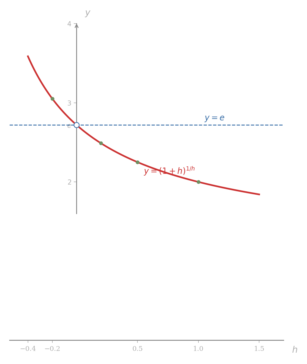
The convergence is slow. At $h = 0.5$ the value of $(1 + h)^{1/h}$ is $(1.5)^{2} = 2.25$ , well below $e$ ; at $h = 0.1$ the value is $(1.1)^{10} \approx 2.594$ ; at $h = 0.01$ the value is $(1.01)^{100} \approx 2.7048$ , still rounded short of $e \approx 2.71828$ in the third decimal.

Continuously Compounded Interest

With $(3)$ in hand, our limit of $(2)$ as $m \to \infty$ follows. Using two of the limit theorems from earlier in the course (the limit of a constant times a function and the limit of a fixed power),

\lim_{m \to \infty} P \!\left(1 + h\right)^{\!(1/h) \cdot r t} = P \!\left[\lim_{h \to 0} (1 + h)^{1/h}\right]^{r t} = P e^{r t}.

Theorem 31 (Continuous compound interest)

A principal of $P$ pounds at annual rate $r$ , compounded continuously for $t$ years, has balance

A(t) = P e^{r t}. \tag{4}

The £ $1000$ at $6\%$ over one year now has a closed-form continuous limit:

1000 \cdot e^{0.06} \approx 1061.84.

This is the upper bound the daily, hourly, and minute-by-minute entries of the table were creeping toward.

The function $A(t) = P e^{r t}$ satisfies the rate equation

A'(t) = r \, A(t), \tag{5}

by the formula for $e^{k x}$ . The proportionality constant in the rate equation $A' = k \, A$ from the solutions theorem is precisely the continuously compounded annual rate $r$ . Interest is being added not at year-end, nor monthly, nor daily, but at every instant, at a rate proportional to whatever is currently in the account.

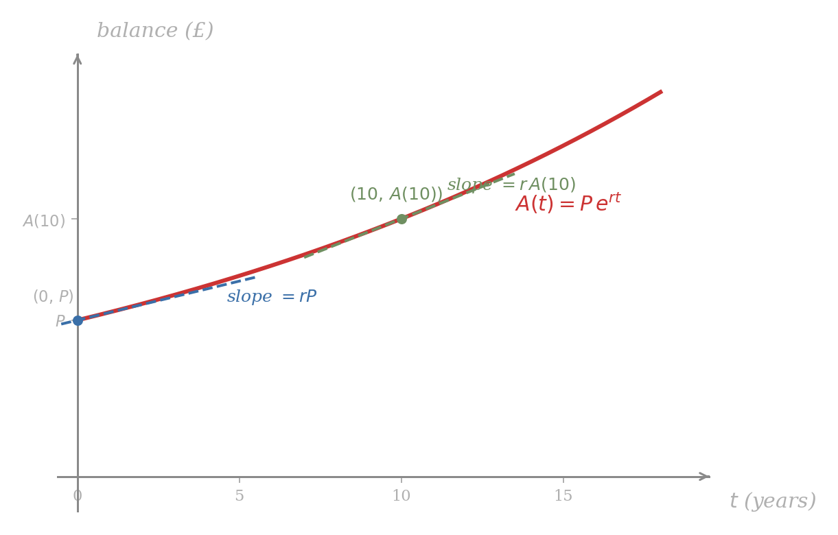
$The continuous compound curve A(t) = Pe^{rt} for P = 1000 and r = 0.05 over 18 years. Two tangent lines are drawn: one at t = 0 with slope rP, and one at t = 10 with slope rA(10), each labelled with its slope. The curve passes through (0, P) and (10, A(10)), both marked.$

The slope at $t = 0$ is $A'(0) = r P$ , which is the simple-interest rate per year applied to the original principal: an account paying continuously at $r$ percent and an account paying simple interest at $r$ percent grow at the same instantaneous rate at $t = 0$ . They diverge for $t > 0$ because the continuous account immediately starts earning on the new interest.

Example 155 (A six-year continuous account)

Recitation 4’s example invested £ $1000$ at $5\%$ per year, compounded annually. Reset the same conditions to continuous compounding at the same nominal rate, and answer four questions about the resulting account.

Write the formula for $A(t)$ .

By $(4)$ with $P = 1000$ and $r = 0.05$ , $A(t) = 1000 \, e^{0.05 \, t}$ .

Find the balance after $6$ years.

$A(6) = 1000 \, e^{0.30} \approx 1349.86$ pounds.

Find the rate at which the balance is growing $6$ years in.

Two routes. The chain rule applied to $(4)$ gives $A'(t) = 1000 \cdot 0.05 \, e^{0.05 \, t} = 50 \, e^{0.05 \, t}$ , so $A'(6) = 50 \, e^{0.30} \approx 67.49$ pounds per year. Alternatively, the rate equation $(5)$ gives the same answer in one step: $A'(6) = 0.05 \cdot A(6) = 0.05 \cdot 1349.86 \approx 67.49$ pounds per year. The growth is in pounds per year because $A$ is in pounds and $t$ is in years.

The $5\%$ advertised rate is not the rate of growth in pounds per year; it is the rate of growth divided by the current balance. Six years in, the £ $1349.86$ balance is itself earning interest, so the growth rate £ $67.49$ /year exceeds the £ $50.00$ /year that the original principal alone would generate.

Find the time at which the initial deposit doubles.

We set $A(t) = 2000$ and solve for $t$ :

1000 \, e^{0.05 \, t} = 2000, \qquad e^{0.05 \, t} = 2.

Taking logarithms by the procedure of Lesson 5PM,

0.05 \, t = \ln 2, \qquad t = \frac{\ln 2}{0.05} \approx 13.86 \text{ years}.

The doubling time depends only on $r$ , not on $P$ . Had the principal been £ $50\,000$ or £ $50$ , the equation $1 = (1/2) \cdot e^{0.05 \, t}$ at the doubling time $t$ collapses to the same $e^{0.05 \, t} = 2$ .

The doubling-time computation in part (d) generalises immediately to any continuously compounded account.

Note (Doubling time at continuous rate $r$)

A continuously compounded account at rate $r > 0$ doubles in time

t_{\mathrm{double}} = \frac{\ln 2}{r}.

The doubling time is independent of the principal $P$ .

Problem 171

A British saver invests £ $P$ at $4\%$ per year compounded continuously.

State $A(t)$ , $A'(t)$ , and the doubling time, all in closed form involving $P$ and $\ln 2$ .
Find the time required for the balance to triple. Express the tripling time as $\ln 3$ times a constant.
Show that the tripling time exceeds the doubling time by exactly $(\ln 3 - \ln 2)/r$ , and rewrite this gap as $\ln(3/2)$ over $r$ using LIII of Lesson 5PM.

Example 156 (Picasso's *The Dream*)

Pablo Picasso’s painting The Dream sold in $1941$ for £ $7\,000$ , a war-distressed price. In $1997$ the painting was auctioned for £ $48.4$ million. Treat the painting as an investment growing under continuous compounding, and find the implied annual rate.

We let $A(t) = P e^{r t}$ measure the value (in millions of pounds) of the painting $t$ years after $1941$ . Then $P = 0.007$ million and $A(56) = 48.4$ million. By $(4)$ ,

0.007 \, e^{56 \, r} = 48.4, \qquad e^{56 \, r} = \frac{48.4}{0.007} \approx 6914.29.

Taking logarithms and applying $(3)$ of Lesson 5PM on the left,

56 \, r = \ln 6914.29, \qquad r = \frac{\ln 6914.29}{56} \approx 0.158.

The painting earned a continuously compounded return of about $15.8\%$ per year over the $56$ -year holding period. Compared to the original Recitation 4 investor at a flat $15\%$ annual return without continuous compounding (so the multiplier is $(1.15)^{56} \approx 2506.6$ , reaching about £ $17.5$ million on the same £ $7\,000$ ), the painting did roughly $2.76$ times better than the same nominal rate compounded only annually. The inferred continuous rate of $15.8\%$ corresponds to an effective annual rate $e^{0.158} - 1 \approx 17.1\%$ , a gap that compounds itself over $56$ years.

Problem 172

A British government war bond issued in $1944$ paid £ $1\,000$ at maturity in $1980$ , after $36$ years. Treating the bond as a continuously compounded investment from a hidden purchase price $P$ at $r = 0.04$ per year, find $P$ in closed form. Verify the closed form against the numerical answer using $\ln 2 \approx 0.693$ and $\ln 5 \approx 1.609$ .

Present Value

Formula $(4)$ takes the principal at time $0$ and projects it forward to time $t$ . The reverse reading takes a target value $A$ to be received at time $t$ and asks how much money invested at time $0$ would grow into that target. We solve $(4)$ for $P$ :

P = A e^{-r t}. \tag{6}

Definition 40 (Present value)

For a future amount $A$ to be received in $t$ years, with money assumed to earn continuous interest at rate $r$ , the present value is

P = A e^{-r t}.

$P$ is the unique principal that, if invested at time $0$ at rate $r$ compounded continuously, would grow exactly into $A$ at time $t$ .

$A continuous compound curve from (0, P) at the left to (T, A) at the right, with the formula A(t) = Pe^{rt} labelling the curve. Two horizontal arrows along the time axis mark the two readings: one above labelled 'compound: A = Pe^{rT}' pointing right, one below labelled 'discount: P = Ae^{-rT}' pointing left.$

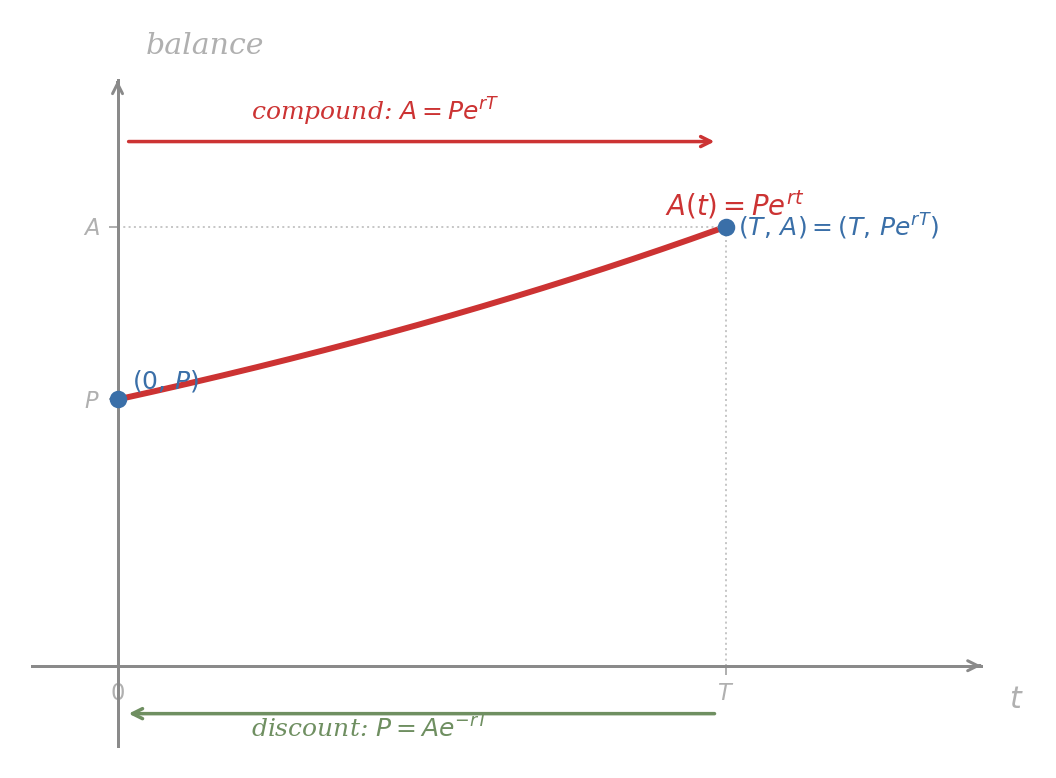
The present value $P$ is what £ $A$ at time $t$ “is worth right now.” Two payments £ $A$ at time $t_{1}$ and £ $A$ at time $t_{2}$ with $t_{1} < t_{2}$ are not equivalent at the same fixed amount, because the second can be matched with less principal today. Present value is the standard exchange rate between money now and money later.

Example 157 (Present value of a deferred payment)

Find the present value of £ $5\,000$ to be received in $2$ years, with money invested at $12\%$ continuous compounding.

By $(6)$ with $A = 5\,000$ , $r = 0.12$ , and $t = 2$ ,

P = 5\,000 \cdot e^{-0.24} \approx 5\,000 \cdot 0.78663 \approx 3933.14 \text{ pounds}.

A holder of £ $3\,933.14$ today, given access to a $12\%$ continuous-compounding account, can convert the present value into the deferred payment with no extra effort: the account grows from £ $3\,933.14$ at $t = 0$ to exactly £ $5\,000$ at $t = 2$ .

Example 158 (Two payment offers)

A British supplier offers two payment terms for the same delivered goods:

Offer A. £ $10\,000$ today.
Offer B. £ $11\,000$ in $18$ months.

The buyer has access to a continuous-compounding account at $r = 0.06$ per year. Which offer is cheaper, and by how much in present-value terms?

Offer A has present value £ $10\,000$ by definition. Offer B has present value, by $(6)$ with $A = 11\,000$ , $r = 0.06$ , and $t = 1.5$ ,

P_{B} = 11\,000 \cdot e^{-0.09} \approx 11\,000 \cdot 0.91393 \approx 10\,053.27 \text{ pounds}.

Offer B is more expensive than Offer A by £ $53.27$ in today’s pounds. Equivalently, the buyer would need to deposit £ $10\,053.27$ today at $6\%$ continuous to clear the £ $11\,000$ in $18$ months.

The threshold rate $r^{\ast}$ at which the two offers tie is the unique $r > 0$ with $11\,000 \, e^{-1.5 \, r} = 10\,000$ . Solving gives $r^{\ast} = (\ln 1.1)/1.5 \approx 0.0635$ , just above the buyer’s $6\%$ . At any rate above $r^{\ast}$ , Offer B is the better deal in present-value terms; at any lower rate, Offer A is.

Remark

A common phrasing in finance is that future payments are “discounted back to the present.” The discount factor for a payment $A$ at time $t$ is $e^{-r t}$ , which is strictly between $0$ and $1$ for every $r > 0$ and $t > 0$ . The further out the payment, the smaller the discount factor, and the smaller the present value of a fixed nominal payment.

Problem 173

A pension fund must pay £ $50\,000$ in $10$ years. Money is invested at $r = 0.04$ per year, compounded continuously.

What present value must the fund hold today to meet the obligation?
If the rate were instead $r = 0.05$ , by what factor would the required present value change? Express the factor as $e^{-0.1}$ and compute it to four decimals.
The fund actually holds £ $30\,000$ today at $r = 0.04$ . How many additional years must elapse before the £ $30\,000$ alone grows into £ $50\,000$ ? Express the answer in closed form involving $\ln(5/3)$ .

Problem 174

A trustee must arrange a payment of £ $M$ in $T$ years. Money is invested at continuous rate $r$ . The trustee may also need to withdraw a fixed amount £ $W$ at an earlier time $\tau$ , with $0 < \tau < T$ , for an unrelated purpose; the withdrawal is removed from the account at $\tau$ and not replaced.

Show that the smallest single deposit $P$ at $t = 0$ that meets both obligations, namely withdrawing £ $W$ at time $\tau$ and still having £ $M$ at time $T$ , is

P = W e^{-r \tau} + M e^{-r T}.

Explain in one sentence why the right side is the sum of the two payments, each discounted to the present at the same rate.

The Effective Annual Rate

Two banks may quote the same nominal rate $r$ but compound at different frequencies. A bank that compounds $m$ times per year multiplies the balance at the end of one year by $(1 + r/m)^{m}$ , while a bank that compounds continuously multiplies it by $e^{r}$ . The convergence figure above showed the latter as the limiting case. The single number that describes the year-on-year multiplier of any compounding scheme is its effective annual rate.

Definition 41 (Effective annual rate)

The effective annual rate of a continuous-compounding scheme at nominal rate $r$ is the unique $R$ for which

1 + R = e^{r}.

Equivalently, $R = e^{r} - 1$ .

A nominal $r = 0.05$ continuous account has effective annual rate $e^{0.05} - 1 \approx 0.05127$ , so an account quoting ” $5\%$ continuous” actually returns about $5.13\%$ per year. The gap widens with $r$ : at $r = 0.10$ , the effective rate is $e^{0.10} - 1 \approx 0.10517$ , and at $r = 0.20$ it is $e^{0.20} - 1 \approx 0.22140$ .

Example 159 (Matching a discrete account to a continuous account)

A British savings account offers $5\%$ per year compounded monthly. Express the same return as a continuous rate.

The discrete-compounding multiplier for one year is $(1 + 0.05/12)^{12}$ . The matching continuous rate $r^{\ast}$ satisfies

e^{r^{\ast}} = (1 + 0.05/12)^{12}.

Take logarithms by Lesson 5PM:

r^{\ast} = 12 \ln \!\left(1 + \frac{0.05}{12}\right) \approx 12 \cdot 0.0041580 \approx 0.04990.

The continuous rate equivalent to monthly compounding at nominal $5\%$ is about $4.99\%$ , slightly less than the nominal $5\%$ . The two accounts produce identical year-end balances, since by construction $e^{r^{\ast}} = (1 + 0.05/12)^{12}$ , but the labels differ because one quotes the continuous rate and the other the nominal.

Problem 175

A bank quotes a nominal annual rate of $r = 0.08$ . Compute the effective annual rate under each compounding scheme: annual ( $m = 1$ ), quarterly ( $m = 4$ ), monthly ( $m = 12$ ), daily ( $m = 360$ ), and continuous. Express each effective rate to four decimal places, and identify the gap between the daily and continuous rates.

Problem 176

The continuous rate matching a stated effective annual rate. A British investor sees an account advertised with effective annual rate $R = 0.07$ . Find the equivalent nominal continuous rate $r$ , in closed form involving $\ln 1.07$ , and verify that the answer is strictly less than $R$ . State a one-sentence reason, in plain words, why $r < R$ is forced.

Two Closing Applications

Our next two examples use the same toolkit on settings where the pattern is what we want, not the closed form.

Example 160 (Continuous beats annual by an exponentially growing factor)

A British investor places £ $P$ at continuous rate $r$ for $n$ years, ending with balance $P e^{r n}$ . A second investor places £ $P$ at the same nominal rate $r$ but compounded only annually, ending with $P (1 + r)^{n}$ . Show that the ratio of the two balances is

\frac{P e^{r n}}{P (1 + r)^{n}} = e^{n \, (r - \ln(1 + r))},

and conclude that the continuous account exceeds the annual account by an exponentially growing factor, with growth constant $r - \ln(1 + r) > 0$ . Find the year at which the continuous balance is twice the annual balance, in closed form involving $r$ .

Our numerator and denominator share the principal $P$ , which cancels. By LIV of Lesson 5PM applied to $(1 + r)^{n}$ ,

(1 + r)^{n} = e^{n \ln(1 + r)},

so the ratio is $e^{r n} / e^{n \ln(1 + r)} = e^{n \, (r - \ln(1 + r))}$ by law (iii) of exponents from Recitation 4. The exponent grows linearly in $n$ at the constant rate $r - \ln(1 + r)$ , which is positive because $\ln(1 + r) < r$ for every $r > 0$ (a fact verified in the next problem from the derivative of $\ln(1 + x) - x$ ).

For the doubling year, we set the ratio equal to $2$ :

e^{n \, (r - \ln(1 + r))} = 2, \qquad n = \frac{\ln 2}{r - \ln(1 + r)}.

At $r = 0.06$ , this gives $n \approx \ln 2 / (0.06 - \ln 1.06) \approx 0.6931 / 0.001731 \approx 400$ years before the continuous account doubles the annual account on the same nominal rate. The gap is real but slow, so everyday savings notation can quote a single annual rate without losing any decimal a saver cares about.

Problem 177

(Harder.) Define $\varphi(x) = \ln(1 + x) - x$ for $x > -1$ . Differentiate $\varphi$ once and show $\varphi'(x) > 0$ for $-1 < x < 0$ and $\varphi'(x) < 0$ for $x > 0$ , so $\varphi$ has a strict relative maximum at $x = 0$ . Conclude $\varphi(x) < \varphi(0) = 0$ for every $x \neq 0$ , that is, $\ln(1 + x) < x$ on $x > -1$ , $x \neq 0$ . Use the inequality, applied at $x = r > 0$ , to confirm the positivity of the growth constant $r - \ln(1 + r)$ in the previous example.

Example 161 (A staggered payment schedule)

A British contractor offers a phased payment plan for the same delivered goods: the buyer pays £ $C$ today, £ $C$ in $1$ year, and £ $C$ in $2$ years, for a total nominal of $3 C$ . The buyer can borrow or lend at continuous rate $r$ . Find the present value of the entire phased plan, then determine the equivalent single-payment-today amount that exactly matches the plan’s present value.

We discount each payment to the present by $(6)$ :

\text{PV} = C + C \, e^{-r} + C \, e^{-2 r}.

The first payment is made at $t = 0$ , so its discount factor is $1$ ; the others use $e^{-r}$ and $e^{-2 r}$ . Pulling $C$ out front gives us

\text{PV} = C \!\left(1 + e^{-r} + e^{-2 r}\right).

At $r = 0.06$ , $e^{-0.06} \approx 0.94176$ and $e^{-0.12} \approx 0.88692$ , so

\text{PV} \approx C \cdot (1 + 0.94176 + 0.88692) = C \cdot 2.82868.

The phased plan with nominal total $3 C$ has present value $2.82868 \, C$ , a reduction of $5.71\%$ from the nominal because two of the three payments earn interest in the buyer’s hands before they are due.

The equivalent single-payment-today amount is exactly the present value $2.82868 \, C$ . A buyer with that amount in hand and access to the $r = 0.06$ account can clear the contractor’s three payments by depositing the lump sum, then withdrawing £ $C$ at each due date.

Problem 178

(Harder.) Two competing British insurance products promise the same payout £ $M$ in $T$ years from a one-time premium $P$ today, but at different continuously compounded rates: product A guarantees rate $r_{A}$ and product B guarantees rate $r_{B} > r_{A}$ . The premia $P_{A}$ and $P_{B}$ are set so that each product just meets its obligation: $P_{A} \, e^{r_{A} T} = M = P_{B} \, e^{r_{B} T}$ .

Express the ratio $P_{A}/P_{B}$ in closed form involving $e^{(r_{B} - r_{A}) T}$ , and conclude that $P_{A} > P_{B}$ .
The buyer’s cost of capital is a third continuous rate $r_{C}$ . The buyer’s effective loss from committing the premium £ $P$ today rather than holding it for $T$ years at rate $r_{C}$ is $P (e^{r_{C} T} - 1)$ . Compute the difference in effective losses between the two products, $\Delta L = (P_{A} - P_{B})(e^{r_{C} T} - 1)$ , and show that $\Delta L > 0$ for every $r_{C} > 0$ .
State, with reasons drawn from this lesson, why the buyer prefers product B on every dimension that matters: smaller premium, smaller effective loss, identical payout.

Problem 179

(Harder.) A real-estate investor purchases a London building for £ $P_{0}$ in year $0$ . The market value $V(t)$ in year $t$ grows under the continuous-compounding model $V(t) = P_{0} \, e^{r \, t}$ . The annual property-tax rate is a continuous outflow of $\alpha \, V(t)$ pounds per year, paid out of the building’s market value. Define the net rate of growth as

\frac{V'(t) - \alpha V(t)}{V(t)}.

Compute the net rate of growth in closed form. Identify it as a constant.
Find the condition on $r$ and $\alpha$ for the net rate of growth to be positive. Express the borderline case as a single equation.
Using this net rate, express the investor’s after-tax doubling time in closed form as $\ln 2$ over a single constant.

Note (Toolkit additions from this lesson)

Rule	Form
Discrete compound interest	$A = P (1 + r/m)^{m t}$
Limit formula for $e$	$\lim_{h \to 0} (1 + h)^{1/h} = e$
Continuous compound interest	$A(t) = P e^{r t}$
Rate equation	$A'(t) = r \, A(t)$
Present value	$P = A \, e^{-r t}$
Doubling time	$t_{\mathrm{double}} = (\ln 2)/r$
Effective annual rate	$R = e^{r} - 1$