
Quantifiers
In Lesson 2, we introduced predicates: expressions like whose truth value depends on the variable substituted. The natural next step is to make claims about all values in a domain, or to assert that at least one satisfying value exists. These are the universal and existential quantifiers, the final logical apparatus for formal mathematical reasoning. But verifying such claims computationally, checking a property across an entire domain or searching until a witness is found, requires a mechanism for repeating instructions. We begin with this mechanism: iteration.
Iteration
At the close of Lesson 2, we established that branching programmes are fundamentally bound by constant time (Definition 36): each instruction is executed at most once, so the total computation is capped by the static length of the source code. The base-expansion algorithm exposed this limitation directly. Each step applied the same pair of operations (// and %) to the current quotient, but without a way to repeat those operations automatically, we wrote every step out by hand. Computing the factorial of , testing whether a number is prime, or extracting the digits of an arbitrarily large base expansion: these are tasks whose duration scales with the input, and no branching programme can accommodate them.
The remedy is iteration: a control structure that redirects execution back to a previously encountered instruction, creating a cycle. Where branching gives us trees, iteration gives us loops.
An iteration (or loop) is a control structure that redirects execution back to a previously encountered instruction, allowing a block of code to be executed repeatedly. The number of repetitions is determined dynamically by the state of the computation, not by the static length of the programme.
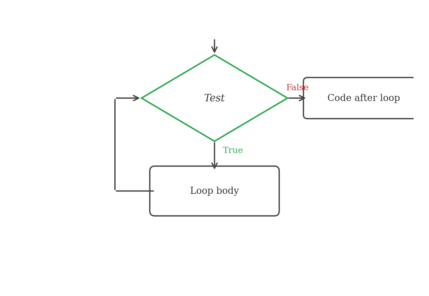
The generic iteration mechanism follows the flowchart below. A logical test is evaluated. If the result is , the interpreter executes a block of instructions called the loop body and returns to re-evaluate the test. This cycle continues until the test evaluates to , at which point control passes to the code following the loop.
The While Loop
Python implements the generic iteration mechanism using the while statement. Its syntax mirrors that of the if statement: a test expression followed by an indented block.
# Structure of a while loop:
# while test:
#     body
When the interpreter reaches a while statement, it evaluates the test. If the test is True, the body executes in full, and control returns to the test. If the test is False, the body is skipped entirely and execution continues with the first statement after the loop.
Consider the following programme, which computes by repeated addition.
x = 3
ans = 0
num_iterations = 0

while num_iterations != x:
    ans = ans + x
    num_iterations = num_iterations + 1

print(f"{x} squared is {ans}")
The code binds x to , then adds x to ans once per iteration, incrementing num_iterations each time. The table below records the value of each variable every time the test num_iterations != x is evaluated. Constructing this table by hand, pretending to be the interpreter and tracing the programme with pencil and paper, is called hand simulation. It is the most reliable method for understanding what a loop actually does.
| Test evaluation | x | ans | num_iterations | Test result |
|---|---|---|---|---|
| 1st | 3 | 0 | 0 | |
| 2nd | 3 | 3 | 1 | |
| 3rd | 3 | 6 | 2 | |
| 4th | 3 | 9 | 3 |
On the fourth evaluation, num_iterations equals x, the test evaluates to False, and the loop terminates. The programme prints 3 squared is 9.
Termination. For what values of x does this programme terminate? There are three cases.
If : the initial value of num_iterations is , so num_iterations != x is immediately False. The body never executes, and the programme prints 0 squared is 0. Correct.
If : the initial value of num_iterations is , so the body executes at least once. Each iteration increases num_iterations by exactly . After exactly iterations, num_iterations equals , the test fails, and the loop terminates. The programme prints the correct value .
If : something goes badly wrong. num_iterations starts at and increases by on each iteration: Since is negative, num_iterations will never equal . The test never evaluates to False, and the programme runs forever. This is an infinite loop.
How do we fix this? Changing the test to num_iterations < abs(x) nearly works: the loop now terminates for negative x, running abs(x) times. But each iteration adds x (a negative number) to ans, producing a negative result. The programme would report (-3) squared is -9. The fix is to also change the body to add abs(x) instead of x:
x = -3
ans = 0
num_iterations = 0

while num_iterations < abs(x):
    ans = ans + abs(x)
    num_iterations = num_iterations + 1

print(f"{x} squared is {ans}")   # -3 squared is 9
Problem 43
The following programme should print the letter X a specified number of times. Replace the comment with a while loop that concatenates 'X' to to_print exactly num_x times.
num_x = int(input('How many times should I print the letter X? '))
to_print = ''
# concatenate X to to_print num_x times
print(to_print)Given a positive integer, its leading digit (or leftmost digit) can be extracted by repeatedly applying floor division by until a single digit remains. We do not know in advance how many digits the number has, so we cannot predict the number of iterations. This is a natural task for a while loop.
n = 72658489290098
n = abs(n)

while n >= 10:
    n = n // 10

print(n)   # 7
Each iteration discards the last digit. The loop terminates when n is a single digit ().
A while loop is the natural choice when the number of iterations is not known before the loop begins. The leading-digit extraction and the squaring fix both illustrate this: the stopping condition depends on the input, and no formula predicts the number of steps needed. When the iteration count is known in advance, a different construct, the for loop (introduced below), is both cleaner and less error-prone.
The Break Statement
It is sometimes convenient to exit a loop without re-evaluating the test at the top. Executing a break statement terminates the loop in which it appears and transfers control immediately to the first statement after the loop.
# Find the smallest positive integer divisible by both 11 and 12
x = 1

while True:
    if x % 11 == 0 and x % 12 == 0:
        break
    x = x + 1

print(x, 'is divisible by 11 and 12')   # 132 is divisible by 11 and 12
The test while True creates a loop that, without a break, would run forever. The break inside the body provides the actual termination condition. This pattern is useful when the exit test is most naturally checked partway through the body rather than at the top.
If a break is executed inside a nested loop (a loop within another loop), only the innermost enclosing loop is terminated. The outer loop continues its own iteration unaffected.
Problem 44
Write a programme that asks the user to input integers (one at a time, using input and int) and then prints the largest odd number entered. If no odd number was entered, it should print a message to that effect.
The For Loop
The while loops above share a common structural pattern: a counter variable is initialised, tested on each iteration, and incremented inside the body. Python provides a dedicated construct, the for loop, that handles this bookkeeping automatically.
The general form is:
# for variable in sequence:
#     code block
The variable following for is bound to the first value in the sequence, and the code block executes. The variable is then assigned the second value, and the block executes again. This continues until the sequence is exhausted or a break is encountered.
total = 0

for num in (77, 11, 3):
    total = total + num

print(total)   # 91
The expression (77, 11, 3) is a tuple, a type of ordered sequence we will study in detail later.
The Range Function
The sequence of values bound to the loop variable is most commonly generated by the built-in range function, which produces a progression of integers. It accepts one, two, or three arguments.
One argument: range(stop) produces .
for i in range(4):
    print(i)

# prints:
# 0
# 1
# 2
# 3
Two arguments: range(start, stop) produces .
# Sum the integers from 5 to 10
total = 0

for x in range(5, 11):
    total = total + x

print(total == 5 + 6 + 7 + 8 + 9 + 10)   # True
Note that range(5, 11) includes but excludes . This half-open convention matches the slicing behaviour of strings (Lesson 2).
Three arguments: range(start, stop, step) produces , stopping before stop.
# Sum every 7th integer from 5 to 20
total = 0

for x in range(5, 21, 7):
    total = total + x

print(total == 5 + 12 + 19)   # True
If step is positive, the last element is the largest integer of the form that is strictly less than stop. If step is negative, the progression descends:
# Sum the odd numbers from 10 down to 4
total = 0

for x in range(10, 3, -1):
    if x % 2 == 1:
        total = total + x

print(total)   # 9 + 7 + 5 = 21
The expression range(40, 5, -10) yields , and range(0, 3) produces the same sequence as range(3). The numbers in the progression are generated on demand, so even range(1000000) consumes negligible memory.
Filtering inside a loop is often cleaner than engineering the step size. The following sums the odd numbers between and regardless of whether itself is odd:
m, n = 4, 10
total = 0

for x in range(m, n + 1):
    if x % 2 == 1:
        total = total + x

print(total) # 5 + 7 + 9 = 21The squaring algorithm from the while loop section can be reimplemented using a for loop. The explicit counter variable and its manual increment disappear entirely:
x = -3
ans = 0

for num_iterations in range(abs(x)):
    ans = ans + abs(x)

print(f"{x} squared is {ans}")   # -3 squared is 9
Unlike the while version, the number of iterations is not controlled by an explicit test, and the index variable num_iterations is not explicitly incremented. The for loop automates both.
Modifying the Index Variable
What happens if the loop variable is reassigned inside the body?
for i in range(2):
    print(i)
    i = 0
    print(i)
This prints 0, 0, 1, 0 and then halts, not an infinite stream of zeros. Before the first iteration, range(2) is evaluated and its first value () is assigned to i. At the start of each subsequent iteration, i is reassigned to the next value in the sequence, regardless of any modifications made inside the body. The sequence produced by range is fixed at the moment the for statement is first reached.
This loop is equivalent to:
index = 0
last_index = 1

while index <= last_index:
    i = index
    print(i)
    i = 0
    print(i)
    index = index + 1
The while version is considerably more cumbersome. The for loop is a convenient linguistic mechanism that eliminates the manual bookkeeping.
Similarly, modifying a variable that was used in the range call has no effect on the loop, because range is evaluated exactly once:
x = 1

for i in range(x):
    print(i)
    x = 4

# prints only: 0
However, if a range call appears in an inner loop, it is re-evaluated each time the inner for statement is reached:
x = 3

for j in range(x):
    print('Outer iteration')
    for i in range(x):
        print('  Inner iteration')
        x = 2
The outer range(x) is evaluated once (when ), so the outer loop runs three times. The inner range(x) is evaluated afresh each time the inner for is reached. On the first pass, , so the inner loop runs three times. On subsequent passes, , so the inner loop runs twice. The total output is three outer iterations and inner iterations:
Outer iteration
  Inner iteration
  Inner iteration
  Inner iteration
Outer iteration
  Inner iteration
  Inner iteration
Outer iteration
  Inner iteration
  Inner iteration
Iterating Over Strings
The for statement combined with the in operator iterates directly over the characters of a string, binding the loop variable to each character in turn:
total = 0

for c in '12345678':
    total = total + int(c)

print(total)   # 36
This sums the digits of the string '12345678' without requiring range or indexing.
Problem 45
Using a for loop and range, compute the sum in two ways: (a) by accumulating in a loop variable, and (b) by verifying against the closed-form formula for the sum of integers from to .
Nested Loops
Placing one loop inside another creates a nested loop. The inner loop runs to completion on every iteration of the outer loop.
The following programme prints an grid of asterisks:
n = 5

for row in range(n):
    for col in range(n):
        print('*', end='')
    print()
Output:
*****
*****
*****
*****
*****
For each value of row, the inner loop runs n times, printing one * per column. The print() after the inner loop moves to a new line.
Modifying the inner loop’s range to depend on the outer variable produces more interesting shapes:
n = 5

for row in range(n):
    print(row, end=' ')
    for col in range(row):
        print('*', end=' ')
    print()
Output:
0
1 *
2 * *
3 * * *
4 * * * *
In the -th row, exactly asterisks appear: a right triangle.
Continue, Break, and Pass
We have already seen break, which terminates the enclosing loop entirely. Two related keywords modify loop control.
continue skips the remainder of the current iteration and returns immediately to the test (for while) or advances to the next value (for for).
pass does nothing at all. It serves as a syntactic placeholder where Python requires a statement but no action is needed.
for n in range(200):
    if n % 3 == 0:
        continue       # skip multiples of 3
    elif n == 8:
        break           # stop entirely at 8
    else:
        pass            # does nothing
    print(n, end=' ')

# prints: 1 2 4 5 7
The numbers are skipped by continue (they are multiples of ). When n reaches , break terminates the loop before print is reached. The values pass through the else branch and reach the print statement.
Primality Testing
We can now tackle a problem that has appeared implicitly since Lesson 1. In that lesson, the proof-system example (Example 3) verified that is composite by exhibiting the divisor , and the verification was a single check: 91 % 7 == 0. But finding the divisor required knowledge we did not justify. With iteration, we can systematically test every candidate.
An integer is prime if its only positive divisors (Definition 37) are and itself: equivalently, no integer in divides . An integer that is not prime is composite.
Translating this directly into a for loop:
n = 91
is_prime = n >= 2

for factor in range(2, n):
    if n % factor == 0:
        is_prime = False
        break

if is_prime:
    print(f'{n} is prime')
else:
    print(f'{n} is not prime')

# 91 is not prime
The loop checks every integer from to . If any divides n, it sets is_prime to False and breaks immediately, since a single witness suffices to establish compositeness. This is a direct computational implementation of the verification procedure from Lesson 1.
We can use this pattern to list all primes below :
for n in range(2, 100):
    is_prime = True
    for factor in range(2, n):
        if n % factor == 0:
            is_prime = False
            break
    if is_prime:
        print(n, end=' ')

# 2 3 5 7 11 13 17 19 23 29 31 37 41 43 47 53 59 61 67 71 73 79 83 89 97
A Faster Primality Test
The programme above checks all potential factors up to , but this is wasteful. If with , then , so . It therefore suffices to check factors up to the largest integer not exceeding (in Python, round(n ** 0.5)). We can also handle separately and then check only odd factors, halving the work again:
n = 1010809
is_prime = n >= 2

if n > 2 and n % 2 == 0:
    is_prime = False
else:
    max_factor = round(n ** 0.5)
    for factor in range(3, max_factor + 1, 2):
        if n % factor == 0:
            is_prime = False
            break

print(f'{n} is prime: {is_prime}')   # 1010809 is prime: True
The difference in speed is substantial. The basic test checks up to candidate factors; the optimised test checks roughly . For , this is the difference between over a million checks and roughly five hundred. We can measure this directly using Python’s time module. (The statement import time loads additional tools built into Python; we will discuss the import mechanism in a later lesson.)
import time

n = 1010809

# Basic primality test
time0 = time.time()
is_prime_basic = True
for factor in range(2, n):
    if n % factor == 0:
        is_prime_basic = False
        break
time1 = time.time()
print(f'Basic: {(time1 - time0) * 1000:.2f} ms')

# Optimised primality test
time0 = time.time()
is_prime_fast = n >= 2
if n > 2 and n % 2 == 0:
    is_prime_fast = False
else:
    max_factor = round(n ** 0.5)
    for factor in range(3, max_factor + 1, 2):
        if n % factor == 0:
            is_prime_fast = False
            break
time1 = time.time()
print(f'Optimised: {(time1 - time0) * 1000:.2f} ms')

print(is_prime_basic == is_prime_fast)   # True
We first verify that both tests agree, then observe the timing gap. On a typical machine, the basic test takes tens of milliseconds while the optimised version completes in a fraction of one.
The -th Element Search
A recurring pattern in computation is finding the -th object satisfying some property. We do not know in advance which integer it will be, so a for loop over a fixed range is inadequate. A while loop is the natural choice: increment a candidate, test whether it has the desired property, and count the successes.
To find the -th positive integer divisible by either or :
target = 5
found = 0
guess = 0

while found <= target:
    guess = guess + 1
    if guess % 4 == 0 or guess % 7 == 0:
        found = found + 1

print(f'The {target}th positive multiple of 4 or 7 (0-indexed) is {guess}')
# The 5th positive multiple of 4 or 7 (0-indexed) is 16
The same pattern extends to any testable property. Combining it with the optimised primality test above, we can locate the -th prime:
target = 10
found = 0
guess = 1

while found <= target:
    guess = guess + 1
    # Optimised primality check (inline)
    is_prime = guess >= 2
    if guess > 2 and guess % 2 == 0:
        is_prime = False
    else:
        max_factor = round(guess ** 0.5)
        for factor in range(3, max_factor + 1, 2):
            if guess % factor == 0:
                is_prime = False
                break
    if is_prime:
        found = found + 1

print(f'The {target}th prime (0-indexed) is {guess}')
# The 10th prime (0-indexed) is 31
We can verify by listing the first few primes: , confirming that the th (counting from ) is indeed .
Problem 46
Write a programme that prints the sum of all prime numbers greater than and less than . You will need a for loop that tests primality nested inside a for loop that iterates over the odd integers between and .
Automating Base Expansions
In Lesson 2, we computed the base- expansion of a natural number by repeatedly applying the Division Theorem (Theorem 9): divide by , record the remainder as the next digit (read right to left), and continue with the quotient until it reaches zero. We observed at the time that “automating this process requires a mechanism for repeating instructions until a condition is met, which we do not yet possess.” We can now fulfil that promise.
n = 12345
b = 17
digits = ''

while n > 0:
    remainder = n % b
    if remainder < 10:
        digits = str(remainder) + digits
    else:
        digits = chr(ord('A') + remainder - 10) + digits
    n = n // b

print(digits)   # 28C3
Each iteration extracts the rightmost digit via n % b and removes it via n // b. The conditional handles digits above by converting them to letters using chr and ord (Lesson 2). Since digits are extracted right to left, each new digit is prepended to the string.
We can verify the result by converting back to decimal:
result = 2 * 17**3 + 8 * 17**2 + 12 * 17 + 3
print(result)   # 12345
This confirms that , matching the hand calculation from Lesson 2 (Example 27).
Problem 47
Modify the base-expansion programme above to handle the case (which should output '0'). Then use it to compute the base- and hexadecimal expansions of , and verify your answers against your hand calculations from Lesson 2 (Problem 37).
Problem 48
Using a while loop and the input function, write a programme that repeatedly asks the user to enter a string. After each entry, it prints the string back to the user. When the user enters 'done', the programme prints 'Bye!' followed by the total number of strings entered (not counting 'done' itself).
Quantification
In Lesson 2, we encountered an argument that propositional logic could not express: “Every prime number greater than is odd. The number is a prime number greater than . Therefore, is odd.” The obstacle was that propositional logic treats each sentence as an indivisible whole and cannot look inside to connect a claim about all primes with a claim about a specific number. With predicates (Definition 15) and the universe of discourse in hand, we now introduce the two symbols that overcome this limitation.
The Universal Quantifier
Let be a predicate with variable ranging over a universe of discourse . The universal quantification of in , written , is the proposition asserting that is for every element . It is read “for all , .”
Determining the truth of amounts to exhaustive verification: examine every object in the universe, and if even one makes false, the entire statement is false. If every object passes, the statement is true. A value for which is called a counterexample.
If the universe is a finite set , the universal quantifier reduces to a conjunction:
When a conjunction or disjunction extends over a collection of terms, we write
More generally, for any index set the notations and denote the conjunction and disjunction, respectively, of over every in . In this notation, the finite-universe equivalences above become and, as we shall see shortly, .
This is precisely what a for loop does. To check computationally, iterate over every element of the domain and test at each step. If the loop completes without finding a counterexample, the universal claim holds. If any element fails, break terminates the loop early:
# Check: is every integer from 1 to 100 positive?
all_hold = True

for x in range(1, 101):
    if not (x > 0):
        all_hold = False
        break

print(all_hold)   # True
The primality test from the previous section is an instance of this pattern: it checks , ” does not divide ”, and breaks on the first counterexample.
Let denote ”.”
If , then is : the value is a counterexample, since is false. If is the positive integers, then is . The truth value of a universally quantified statement depends on the choice of universe.
The Existential Quantifier
Let be a predicate with variable ranging over a universe . The existential quantification of in , written , is the proposition asserting that there is at least one element for which is . It is read “there exists an such that .”
Where the universal quantifier demands exhaustive verification, the existential quantifier demands a search: examine objects in the universe until one satisfies . If such an object is found, it is called a witness and the statement is true. If the entire universe is exhausted without finding a witness, the statement is false.
If the universe is finite:
Computationally, this is again a for loop, but now searching for a single success rather than checking all:
# Check: does there exist an integer from -5 to 5 that is negative?
witness_found = False

for x in range(-5, 6):
    if x < 0:
        witness_found = True
        break

print(witness_found)   # True
If is true and is non-empty, then must also be true: if every element satisfies , at least one does.
Let denote ”.”
is when (witness: ), when is the positive integers, and when is the negative integers.
The following table summarises the two quantifiers:
| Statement | True when | False when |
|---|---|---|
| is for every | There exists a counterexample: some with | |
| There exists a witness: some with | is for every |
If the domain is finite, quantifiers are technically unnecessary: is a conjunction and is a disjunction, both expressible in propositional logic. The power of quantifiers lies in their ability to make claims about infinite domains, where no finite conjunction or disjunction suffices.
Scope and Variable Binding
The scope of a quantifier is the portion of the formula to which it applies, typically delimited by parentheses. A variable that falls within the scope of a quantifier is bound to that quantifier. A variable not bound by any quantifier is free. A formula with free variables is a predicate (Definition 15), not a proposition (Definition 1); it becomes a proposition only when all free variables are either substituted by terms or bound by quantifiers.
Quantifiers bind more tightly than all propositional connectives. Consequently:
This expression has a free variable in and is therefore a predicate, not a proposition. The two ‘s are in fact independent: the expression could equivalently be written . By contrast, binds both occurrences of and is a proposition.
The Unique Existential Quantifier
It is often useful to assert that exactly one object satisfies a predicate.
The unique existential quantification asserts that exactly one element of satisfies . It is defined in terms of the other quantifiers:
This reads: “there exists an such that , and any satisfying must equal .”
Let denote "" with . Then is : the unique witness is . If instead denotes "" over , then is , since infinitely many positive integers exist.
Formalising Arguments
We can now symbolise the prime-number argument that propositional logic could not handle. Let denote ” is a prime number greater than ” and denote ” is odd.”
- “Every prime number greater than is odd” becomes .
- “The number is a prime number greater than ” becomes .
- By substituting into (1) we obtain . Since is true by (2) and the conditional is true, bivalence forces to be true: ” is odd.”
The deduction is no longer blocked by syntactic limitations.
More broadly, the four classical categorical propositions of Aristotelian logic can be expressed in first-order form. Given predicates and :
| Type | Statement | First-order form |
|---|---|---|
| A | All are | |
| E | No is | |
| I | Some is | |
| O | Some is not |
Note the use of in the universal forms versus in the existential forms. A common error is to write , which makes the much stronger claim that everything in the universe is both and . Equally, is almost always vacuously true: any element that is not makes the implication true and serves as a witness.
Let denote ” is a student in this class” and denote ” has written a programme in Python.” Let be all people.
“Every student in this class has written a programme in Python” is formalised as .
“Some student in this class has written a programme in Python” is formalised as .
Note the connective change: for the universal, for the existential.
We can verify such statements computationally. Suppose we have a small universe of five students, with a string recording whether each has written a programme ('Y' or 'N'):
# Student IDs 0 through 4; wrote_python[i] is 'Y' if student i has written a programme
wrote_python = 'YYNYY'

# ∀x (S(x) → P(x)): has every student written a programme?
all_wrote = True
for x in range(5):
    if wrote_python[x] != 'Y':
        all_wrote = False
        break
print(f'All wrote Python: {all_wrote}')   # False (student 2 did not)

# ∃x (S(x) ∧ P(x)): has at least one student written a programme?
some_wrote = False
for x in range(5):
    if wrote_python[x] == 'Y':
        some_wrote = True
        break
print(f'Some wrote Python: {some_wrote}')   # True (student 0)
Quantifier Negation
The universal and existential quantifiers are duals, connected by negation in a manner analogous to De Morgan’s laws for conjunction and disjunction.
For any predicate with universe :
(1)
(2)
(1) By definition, asserts that is true for every . Equivalently, it is the conjunction
Negating and applying De Morgan’s law (extended to possibly infinite conjunctions):
(2) Similarly, . Negating:
■As immediate consequences: and .
# Demonstrating quantifier negation over {-2, -1, 0, 1, 2}
# ¬(∀x: x > 0)  should equal  ∃x: x ≤ 0

all_positive = True
for x in range(-2, 3):
    if not (x > 0):
        all_positive = False
        break

exists_non_positive = False
for x in range(-2, 3):
    if x <= 0:
        exists_non_positive = True
        break

# The negation of the universal equals the existential of the negation
print((not all_positive) == exists_non_positive)   # True
Shorthand Notation
When the universe of discourse is restricted to a specific set , we write:
This notation is coherent with negation. Applying the quantifier negation theorem:
The restricted domain is preserved under negation: only the predicate is negated, not the domain condition.
Distribution of Quantifiers over Connectives
The universal quantifier distributes over conjunction, and the existential quantifier distributes over disjunction:
However, the reverse pairings do not hold in general:
For both non-equivalences, a single counterexample suffices. Let denote ” is even” and denote ” is odd” over . Then is (witness for , witness for ), but is (no integer is both even and odd). Similarly, is (every integer is even or odd), but is (not every integer is even, and not every integer is odd).
Validity and Satisfiability in Predicate Logic
Just as in propositional logic (Lesson 1), a quantified statement with all variables bound can be classified by its truth behaviour across all possible interpretations. A statement is valid if it is true for every domain and every choice of predicates (the analogue of a tautology). It is satisfiable if there exists at least one domain and choice of predicates making it true, and unsatisfiable if no such choice exists.
The statement is valid: it is an instance of the quantifier negation theorem and holds for any predicate and any domain.
The statement is satisfiable: taking makes it true, but choosing and over makes it false.
The statement is unsatisfiable: it asserts that every element simultaneously satisfies and fails to satisfy , contradicting the Principle of Bivalence (Lesson 1).
Problem 49
Determine whether each of the following statements is valid, satisfiable, or unsatisfiable. Justify your answer.
(a)
(b)
(c)
Problem 50
Let , and denote ” is a clear explanation”, ” is satisfactory”, and ” is an excuse” respectively, with the domain being all English texts. Formalise the following in predicate logic:
(a) All clear explanations are satisfactory.
(b) Some excuses are unsatisfactory.
(c) Some excuses are not clear explanations.
Problem 51
Using the quantifier negation theorem, negate each of the following statements and simplify. State whether the original or its negation is true.
(a)
(b)
(c)
Nested Quantifiers
The statements encountered so far have involved a single quantifier binding a single variable. Many mathematical claims, however, involve multiple variables and require several quantifiers applied in sequence. A nested quantifier is a quantifier that falls within the scope of another quantifier.
The statement “every real number has an additive inverse” involves two variables: the number itself and its inverse. With , the formalisation is:
The outer quantifier asserts that the claim holds for every . The inner quantifier asserts that, for each such , a suitable exists. The two quantifiers are nested: lies within the scope of .
We can verify this computationally over a finite domain. Each nested quantifier corresponds to a nested loop: the outer for loop iterates over , and the inner for loop searches for a witness :
# Check: ∀x ∃y (x + y == 0) over {-3, -2, ..., 3}
domain = range(-3, 4)
result = True

for x in domain:
    found_inverse = False
    for y in domain:
        if x + y == 0:
            found_inverse = True
            break
    if not found_inverse:
        result = False
        break

print(result)   # True
A nested quantified statement can be decomposed by treating each inner quantification as a propositional function. For instance, can be read as , where and . Note that is itself a predicate: the existential quantifier binds , but remains free until the outer binds it.
Order of Quantifiers
The order in which quantifiers appear is critical. Consider the same predicate over .
asserts: “for every , there exists a such that .” This is : for any given , the witness works. Crucially, the witness may differ for each .
asserts: “there exists a single such that for every .” This is : no single number is the additive inverse of every real number.
The computational difference is visible in the loop structure:
# ∃y ∀x (x + y == 0): does a single y work for all x?
domain = range(-3, 4)
result = False

for y in domain:
    works_for_all = True
    for x in domain:
        if x + y != 0:
            works_for_all = False
            break
    if works_for_all:
        result = True
        break

print(result)   # False
In the first programme (), the outer loop iterates over and the inner loop searches for a fresh at each step. In the second (), the outer loop searches for a single and the inner loop tests whether it works for every . The quantifier order dictates which variable the outer loop controls.
However, quantifiers of the same type may be freely reordered:
Both nested universal quantifiers demand that hold for every pair, and both nested existential quantifiers demand that at least one pair satisfies . In neither case does the order in which pairs are examined affect the outcome.
The statement “the sum of two positive integers is always positive” contains implicit quantifiers and a hidden domain. Making these explicit step by step:
- Rewrite with explicit quantifiers: “for every two integers, if both are positive, then their sum is positive.”
- Introduce variables: “for all integers and , if and , then .”
- Formalise with :
Note the use of rather than : the universal quantifier ranges over all integers, and the implication restricts attention to those that are positive (Type A categorical form, as in the table above).
Let denote ” loves ”, with being all people.
Observe how the English phrasing obscures the quantifier order. “Everybody loves somebody” places the universal quantifier first (): each person has their own someone. “There is someone who is loved by everyone” places the existential first (): a single person is loved by all. Despite their superficial similarity, the two statements are logically independent.
Problem 52
Let denote ” and are friends” with the domain being all students in a class. Formalise the following in predicate logic:
(a) Everyone has a friend.
(b) There is someone who is friends with everyone.
(c) No one is friends with everyone.
(d) There exists a pair of students who are not friends with each other.
Determine the truth value of each statement, where :
(a) is : for any , choose .
(b) is : taking , there is no real with .
(c) is : choose .
(d) is : addition over is commutative, so for all . This is the negation of , which is .
Problem 53
Determine the truth value of each statement, where . Justify your answer.
(a)
(b)
(c)
Negating Nested Quantifiers
The quantifier negation theorem (Theorem 11) extends to nested quantifiers by repeated application. Each quantifier flips () and the negation pushes inward:
At each step, one quantifier is negated. The process terminates when the negation reaches the predicate.
Negate the statement (“every real number has an additive inverse”).
Applying the negation rules from outside in:
In English: “there exists a real number with no additive inverse.” Over this is , confirming the original statement is .
Problem 54
Negate each of the following statements and simplify. State whether the original or its negation is true.
(a) , where
(b) , where
(c) , where
A formula is in Prenex Normal Form (PNF) if all quantifiers appear at the front, followed by a quantifier-free predicate:
where each is either or , and contains no quantifiers. For example, the statement is not in PNF because quantifiers appear on both sides of . Rewriting using the conditional equivalence (Lesson 1) and renaming variables for clarity:
The last expression is in PNF. Every statement in predicate logic can be converted to PNF using quantifier negation, variable renaming, and the distribution rules established earlier.
Problem 55
Convert the following to Prenex Normal Form:
(a)
(b)