
Lesson assets
No linked assets.
Search and Approximation
In the AM session, we introduced iteration and used it to verify quantified statements by exhaustive checks over a domain. The primality test asked: does there exist a divisor of in ? The universal check asked: does every element of a domain satisfy some predicate? In each case, the loop served as a computational implementation of a quantifier, scanning the domain one element at a time.
In this recitation, we push the idea further. Instead of merely checking whether a value with a given property exists, we use loops to find it. The shift from verification to search is where iteration becomes powerful, and it brings with it new questions: how do we guarantee that a search terminates? How quickly does it converge? And what happens when the arithmetic itself introduces errors?
Exhaustive Enumeration
The simplest search strategy is the one we have already seen in the context of quantifiers: try every candidate in some domain until one works. When the domain is finite (or can be made finite by restricting attention to a bounded range), this approach is called exhaustive enumeration, and it is guaranteed to find a solution if one exists.
Cube Roots
Suppose we want to find the integer cube root of a perfect cube. Given an integer , we seek an integer such that , or wish to report that no such integer exists.
The strategy is direct: test in order until either (success) or (failure, since implies for positive integers). For negative , the cube root is the negation of the cube root of .
n = 27
x = 0

while x ** 3 < abs(n):
    x = x + 1

if x ** 3 != abs(n):
    print(f'{n} is not a perfect cube')
else:
    if n < 0:
        x = -x
    print(f'Cube root of {n} is {x}')

# Cube root of 27 is 3
Hand simulation for :
| Iteration | x | x ** 3 | x ** 3 < 27 |
|---|---|---|---|
| Start | 0 | 0 | |
| 1 | 1 | 1 | |
| 2 | 2 | 8 | |
| 3 | 3 | 27 |
The loop terminates when , and since , the programme reports success.
Problem 1
Tracing cube roots. The programme above searches for an integer cube root by incrementing x from . Trace the execution for , , and : in each case, construct the hand-simulation table, state the value of x when the loop terminates, and determine whether the programme reports a perfect cube.
How fast is exhaustive enumeration in practice? Try . The cube root is (since ), so the loop iterates times. On a modern machine, this completes almost instantaneously. Now try . The cube root is , so the loop runs nearly two million times, yet the programme still finishes in under a second. Modern processors execute billions of instructions per second; a million iterations is negligible.
Termination and Decrementing Functions
Every loop in a correct programme must eventually terminate (unless it is intentionally infinite, such as a server’s event loop). To prove termination rigorously, we exhibit a quantity that strictly decreases on each iteration and is bounded below.
A decrementing function for a loop is an integer-valued expression of the programme variables such that:
- whenever the loop test evaluates to , and
- strictly decreases on every iteration of the loop body.
If a loop admits a decrementing function, it terminates after at most iterations, where is the initial value of .
The existence of a decrementing function converts the informal assertion “this loop eventually stops” into a rigorous mathematical argument. For the cube-root search, the natural candidate is : it starts non-negative, and each iteration reduces it by .
But this uses a notation we have not yet formalised. In Homework 2 (Problem 12), we introduced the floor function , the greatest integer less than or equal to . Its companion rounds upward.
The ceiling of a real number , written , is the least integer greater than or equal to . Equivalently, .
For example, , , and . The floor and ceiling of satisfy , with equality on both sides precisely when is an integer.
The exhaustive cube-root search terminates for every non-negative integer .
Define . Initially , so . Whenever the loop test holds, we have , giving . Each iteration increments by , so decreases by exactly . Since is a non-negative integer that decreases by per iteration, the loop executes at most times.
■When a programme appears to run forever, the decrementing-function framework suggests a diagnostic strategy. Identify the quantity that should be decreasing. If you cannot find one, the loop may lack a valid decrementing function, which is the mathematical signature of a potential infinite loop. Print the candidate decrementing function at each iteration; if the printed values fail to decrease, the bug is in the loop body. For example, commenting out x = x + 1 in the cube-root search gives on every iteration, constant rather than decreasing.
Exhaustive enumeration is correct and simple, but it can be slow. The cube-root search tests candidates. For , that is iterations: entirely manageable. For , it is iterations, which could take minutes or hours. We shall shortly see a method that reduces steps to roughly .
Approximate Solutions
The cube-root search works only for perfect cubes: it demands an exact integer answer. But many numerical problems have no exact answer in the integers, or even in the rationals. The square root of is irrational, If we insist on exactness, no finite programme can return . The remedy is to relax the requirement: instead of the exact root, we seek a value close enough.
Let be a function and a target value. An -approximation to a solution of is a value such that , where is a prescribed tolerance.
The idea is to accept a controlled amount of error. The tolerance is chosen by the programmer: a smaller demands a more accurate answer but, as we shall see, may require vastly more computation.
Exhaustive Search for Square Roots
We adapt exhaustive enumeration to the approximate setting. Instead of testing integers , we test values where is a small step size. For each candidate , we check whether .
n = 25
epsilon = 0.01
step = 0.0001
guess = 0.0
num_guesses = 0

while abs(guess ** 2 - n) >= epsilon and guess <= n:
    guess = guess + step
    num_guesses = num_guesses + 1

if abs(guess ** 2 - n) >= epsilon:
    print(f'Failed to find sqrt({n})')
else:
    print(f'{guess} is close to sqrt({n})')
    print(f'Number of guesses: {num_guesses}')

# 4.9999... is close to sqrt(25)
# Number of guesses: ~49990
The programme tests roughly candidates before reaching the neighbourhood of . For and , that is up to candidates. The result is not exactly, but that is by design: is within of the true root, which is all we asked for.
Consider the same programme with :
n = 0.25
epsilon = 0.01
step = 0.0001
guess = 0.0

while abs(guess ** 2 - n) >= epsilon and guess <= n:
    guess = guess + step

if abs(guess ** 2 - n) >= epsilon:
    print(f'Failed to find sqrt({n})')

# Failed to find sqrt(0.25)
The search fails because , but the loop condition guess <= n halts the search at , well before reaching . The guard was designed for , where . For , we have , so the upper bound must be adjusted.
Now try with the same step . The programme runs for a long time and eventually reports failure. The step size is too large: the algorithm steps over every value close to without landing within of the true root. Making smaller (say ) fixes the problem, but the programme must then test roughly candidates. We could try to speed things up by starting closer to the answer, but that presumes we already know the neighbourhood of the answer.
There is a deeper tension at work. The step size controls both the accuracy of the answer and the running time. A smaller gives a more precise result but requires more iterations. We need a fundamentally better strategy.
Bisection Search
The key observation is that exhaustive enumeration ignores information. Each failed guess tells us whether was too small or too large, but we discard this knowledge and blindly proceed to . A cleverer strategy would use the comparison to eliminate half the remaining candidates at each step.
This is exactly what you do when looking up a word in a dictionary. You do not start at page one and scan every entry. You open the dictionary near the middle. If the word you seek comes after the visible page, you discard the first half; otherwise, you discard the second half. You then repeat on the surviving half, halving the search space each time.
Before stating the algorithm precisely, we fix notation for the sets it operates on.
For real numbers , we write (reading as “the set of all real such that ”):
- , a closed interval,
- , an open interval,
- and , half-open intervals.
The notation for an open interval is standard but potentially ambiguous with the ordered pair . Context resolves the ambiguity; where confusion is possible, the continental notation is sometimes used.
Bisection search (or binary search) solves on an interval where preserves order (that is, implies throughout), by maintaining the invariant that the solution lies within and repeatedly halving the interval:
- Compute the midpoint .
- If is too large, set . If is too small, set .
- Repeat until or the interval is sufficiently narrow.
After steps, the interval has width , where is the initial width.
The narrowing interval in bisection search is an early instance of a pattern that recurs throughout analysis: a sequence of values approaching a target, with the error shrinking by a predictable factor at each step. We will formalise this idea under the name convergence when we study sequences and limits.
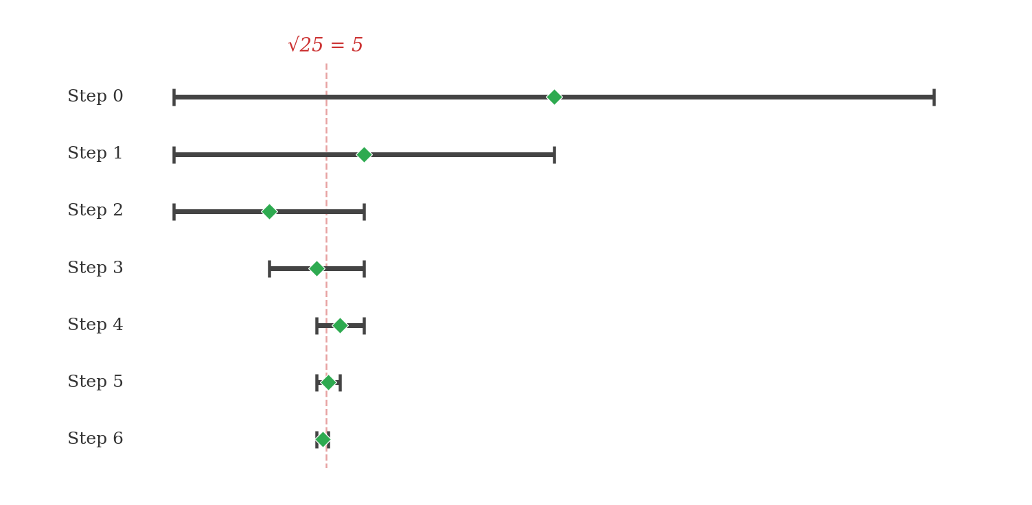
The figure below traces bisection search for on the interval . Each row shows one iteration: the grey bar is the surviving interval, the green diamond marks the midpoint, and the dashed red line marks the true root at .
Implementation
n = 25
epsilon = 0.01
low = 0.0
high = max(1.0, n)
guess = (low + high) / 2.0
num_guesses = 0

while abs(guess ** 2 - n) >= epsilon:
    num_guesses = num_guesses + 1
    if guess ** 2 < n:
        low = guess
    else:
        high = guess
    guess = (low + high) / 2.0

print(f'{guess} is close to sqrt({n})')
print(f'Number of guesses: {num_guesses}')

# 4.999923706054... is close to sqrt(25)
# Number of guesses: 13
Where exhaustive enumeration needed roughly guesses, bisection needs . Note the use of max(1.0, n) for the upper bound: Python’s built-in max returns the larger of its arguments (Homework 2, Problem 4), so this ensures that lies within whether or , correcting the failure we observed with exhaustive approximation.
Tracing the first four steps for on :
| Step | low | high | guess | guess ** 2 | Action |
|---|---|---|---|---|---|
| 0 | 0.0 | 25.0 | 12.5 | 156.25 | Too high: high = 12.5 |
| 1 | 0.0 | 12.5 | 6.25 | 39.0625 | Too high: high = 6.25 |
| 2 | 0.0 | 6.25 | 3.125 | 9.765625 | Too low: low = 3.125 |
| 3 | 3.125 | 6.25 | 4.6875 | 21.972656 | Too low: low = 4.6875 |
After four steps, the interval has shrunk from width to width . Four more steps reduce it to roughly .
Recall that exhaustive approximation failed on because the step size was either too large (missing the root) or too small (requiring hundreds of millions of guesses). Bisection search handles it effortlessly. The initial interval is , and bisection needs roughly guesses. Running the programme confirms: it terminates in guesses (the slight excess over the bound comes from testing rather than the interval width).
Convergence
The bisection algorithm produces a sequence of guesses that draw progressively closer to the true root. Each step halves the interval containing the root, so the distance between the guess and the true answer shrinks by a factor of at every iteration. This is an instance of a general phenomenon, a sequence of values approaching a target, which we will later study under the name convergence. For now, we establish the rate at which bisection approaches its target.
The bound involves the logarithm base , written : the power to which must be raised to produce . For example, since , and since . For values that are not exact powers of , is not an integer; for instance, .
Let be the initial interval and the desired tolerance. Bisection search terminates after at most iterations.
After iterations, the interval has width . The midpoint of an interval of width is within of any point in the interval, so the guess is within of the true root. We need , which gives , hence . The smallest integer satisfying this is .
■For on with :
The bound predicts at most iterations. Our programme used (the slight discrepancy arises because the termination test checks rather than the interval width directly, and floating-point rounding can add an extra step).
Exhaustive enumeration with step tests roughly candidates. Bisection search tests roughly candidates. To appreciate the difference concretely: for and tolerance , exhaustive enumeration would need on the order of guesses, while bisection needs roughly . Every time the search range doubles, exhaustive enumeration doubles its work; bisection adds a single extra step. This is the power of halving: even for astronomically large ranges, the number of bisection steps remains modest.
Problem 2
Bisection for cube roots. The bisection programme above approximates by checking whether guess ** 2 overshoots or undershoots . Adapt it to approximate to within . How many guesses does your programme require? Compare this to the number of steps exhaustive enumeration with step would need.
Machine Arithmetic
The approximate methods above assume that arithmetic on real numbers is exact: that equals , that halving an interval truly halves it, and that the only source of error is the deliberate tolerance . On a computer, these assumptions are false.
Binary Fractions
Computers store numbers in binary. Just as the decimal system represents fractions using negative powers of , so that , the binary system uses negative powers of :
The decimal fraction has an exact binary representation:
Similarly, and . These fractions are exact because their denominators are powers of : , , .
But not every decimal fraction is so accommodating.
The fraction has no finite binary representation.
Suppose for contradiction that for some finite sequence of bits . Then
for some non-negative integer . This gives , so is divisible by . But is a power of , and since is an odd prime, for any . This contradicts .
■This is not a quirk of the number . A rational number in lowest terms has a finite binary expansion if and only if is a power of . Since , the fraction requires an infinite repeating binary expansion, just as repeats infinitely in decimal.
Floating-Point Consequences
Python’s float type stores numbers using the IEEE 754 double-precision format: bits encoding a sign, an -bit exponent, and a -bit significand (plus one implied leading bit). This provides approximately to significant decimal digits of precision.
The practical consequence is that decimal constants which look exact in source code are silently rounded to the nearest representable binary fraction. We can expose this by using the format specifier :.20f inside an f-string, which prints digits after the decimal point:
print(0.1)              # 0.1  (display is rounded)
print(f'{0.1:.20f}')    # 0.10000000000000000555

print(0.1 + 0.1 + 0.1 == 0.3)    # False
print(f'{0.1 + 0.1 + 0.1:.20f}') # 0.30000000000000004441
print(f'{0.3:.20f}')              # 0.29999999999999998890
The sum is not : it overshoots by approximately . Meanwhile, the literal 0.3 is itself rounded downward from the true . The two rounding errors go in opposite directions, so == returns False.
Consider the following attempt to count from to in steps of :
x = 0.0
count = 0

while x != 1.0:
    x = x + 0.1
    count = count + 1
    if count > 20:
        print('Gave up')
        break
This loop never terminates naturally. After additions of , x is , not . The eleventh addition overshoots to , so x skips past entirely. The equality test x != 1.0 is never satisfied. Replacing != with < 1.0 or abs(x - 1.0) < epsilon resolves the issue.
Never test floating-point numbers for exact equality. The expression x == 0.3 is almost certainly wrong, even if x was computed by a formula that is mathematically equal to . Instead, test whether the difference is small:
x = 0.1 + 0.1 + 0.1
print(abs(x - 0.3) < 1e-9)   # True
This is precisely the -approximation philosophy applied to equality testing. The tolerance should reflect the precision of the computation, not the precision of the display.
Suppose we sum one thousand times:
total = 0.0

for i in range(1000):
    total = total + 0.1

print(f'{total:.20f}')    # not exactly 100.0
print(total == 100.0)      # False
print(abs(total - 100.0))  # small but nonzero
Each addition introduces a rounding error of roughly . Over additions, these errors accumulate to roughly : small in absolute terms, but enough to defeat an exact equality test.
For the bisection search above, floating-point error is harmless: we already expect an approximate answer, and the tolerance is vastly larger than the rounding errors. The danger arises when code implicitly assumes exact arithmetic, for instance by testing x == 0.0 instead of abs(x) < epsilon, or by relying on a loop counter that increments by 0.1 to hit exactly 1.0 after ten steps.
Exercises
Exercise 1 (Quantifier Ordering)
Let denote the predicate ” is even,” where and range over the integers. The order in which quantifiers appear determines the meaning of a statement; exchanging and can change a true statement into a false one.
(a) Prove that is true.
(b) Prove that is false.
Exercise 2 (Distribution and Pigeonhole)
You have indistinguishable marbles, , and indistinguishable bags.
(a) What is the smallest value of such that any distribution of marbles into bags is guaranteed to produce either marbles in the same bag or bags each containing at least one marble? Prove your answer.
(b) Now suppose there are marbles and bags, where and are positive integers. Prove that there is a unique way to distribute the marbles such that the number of marbles in any two bags differs by at most one.
Exercise 3 (Parametric Uniqueness)
Consider the equation , where .
(a) Show that the following statement is false: for all , there is a unique such that .
(b) Find the set of real numbers such that the following statement is true: for all , there is a unique such that .
Exercise 4 (Even-Indexed Extraction)
Strings in Python are indexed starting from , so the even-indexed characters of a string s occupy positions Given a string variable my_str, write a programme that prints a new string containing the even-indexed characters of my_str. For example, if my_str = "abcdefg", the output should be aceg.
Exercise 5 (Bisection Guessing)
Suppose you are given an integer with . Write a programme that uses bisection search to determine . The programme should print two lines: count: followed by the number of guesses needed, and answer: followed by the value of . If the midpoint of the current interval falls exactly between two integers, choose the smaller one.
Exercise 6 (Perfect Power Decomposition)
A positive integer is a perfect power if for some integers and . Write a programme that reads a positive integer and prints integers root and pwr satisfying and . If no such pair exists, print a message to that effect.
Test on (which admits , , and ), (), and (not a perfect power with exponent below ).
Exercise 7 (Logarithm by Bisection)
The logarithm base of a positive real number is the value satisfying . Write a programme that uses bisection search to approximate to within . Your programme must first determine an interval guaranteed to contain : note that , and grows without bound as increases, so such an interval can always be found. Test on (), (), and .